Métodos para reducir la pérdida sanguínea durante la resección hepática: un metanálisis en red
Appendices
Appendix 1. Search strategies
| Database | Time span | Search strategy |
| The Central Register of Controlled Trials (CENTRAL) | 2015, Issue 9 | 1. Blood loss OR bleeding OR hemorrhage OR haemorrhage OR hemorrhages OR haemorrhages OR hemostasis OR haemostasis OR transfusion 11. MeSH descriptor Hepatectomy explode all trees 12. (9 OR 10 OR 11) |
| MEDLINE (PubMed) | January 1947 to September 2015 | (Blood loss OR bleeding OR hemorrhage OR haemorrhage OR hemorrhages OR haemorrhages OR hemostasis OR haemostasis OR transfusion OR "Hemorrhage" [MeSH] OR "Blood Transfusion" [MeSH]) AND (((liver OR hepatic OR hepato* OR "liver" [MeSH]) AND (resection OR resections OR segmentectomy OR segmentectomies)) OR hepatectomy OR hepatectomies OR "hepatectomy" [MeSH]) AND ((randomized controlled trial [pt] OR controlled clinical trial [pt] OR randomized [tiab] OR placebo [tiab] OR drug therapy [sh] OR randomly [tiab] OR trial [tiab] OR groups [tiab]) NOT (animals [mh] NOT humans [mh])) |
| Embase (OvidSP) | January 1974 to September 2015 | 1. (Blood loss or bleeding or hemorrhage or haemorrhage or hemorrhages or haemorrhages or hemostasis or haemostasis or transfusion).af 12. (Random* OR factorial* OR crossover* OR cross over* OR cross‐over* OR placebo* OR double* adj blind* OR single* adj blind* OR assign* OR allocat* OR volunteer*).af 13. 11 OR 12 14. 10 AND 13 |
| Science Citation Index Expanded (Web of Science) | January 1945 to September 2015 | 1. TS=(Blood loss OR bleeding OR hemorrhage OR haemorrhage OR hemorrhages OR haemorrhages OR hemostasis OR haemostasis OR transfusion) |
| World Health Organization International Clinical Trials Registry Platform Search Portal (www.who.int/ictrp) | September 2015 | Liver resection OR hepatectomy |
Appendix 2. WinBUGS code
Binary outcome
Binary outcome ‐ fixed‐effect model
# Binomial likelihood, logit link
# Fixed effects model
model{ # *** PROGRAM STARTS
for(i in 1:ns){ # LOOP THROUGH trials
mu[i] ˜ dnorm(0,.0001) # vague priors for all trial baselines
for (k in 1:na[i]) { # LOOP THROUGH ARMS
r[i,k] ˜ dbin(p[i,k],n[i,k]) # binomial likelihood
# model for linear predictor
logit(p[i,k]) <‐ mu[i] + d[t[i,k]] ‐ d[t[i,1]]
# expected value of the numerators
rhat[i,k] <‐ p[i,k] * n[i,k]
#Deviance contribution
dev[i,k] <‐ 2 * (r[i,k] * (log(r[i,k])‐log(rhat[i,k]))
+ (n[i,k]‐r[i,k]) * (log(n[i,k]‐r[i,k]) ‐ log(n[i,k]‐rhat[i,k])))
}
# summed residual deviance contribution for this trial
resdev[i] <‐ sum(dev[i,1:na[i]])
}
totresdev <‐ sum(resdev[]) # Total Residual Deviance
d[1]<‐0 # treatment effect is zero for reference treatment
# vague priors for treatment effects
for (k in 2:nt){ d[k] ˜ dnorm(0,.0001) }
# pair wise ORs and LORs for all possible pair‐wise comparisons, if nt>2
for (c in 1:(nt‐1)) {
for (k in (c+1):nt) {
or[c,k] <‐ exp(d[k] ‐ d[c])
lor[c,k] <‐ (d[k]‐d[c])
}
}
# ranking on relative scale
for (k in 1:nt) {
# rk[k] <‐ nt+1‐rank(d[],k) # assumes events are “good”
rk[k] <‐ rank(d[],k) # assumes events are “bad”
best[k] <‐ equals(rk[k],1) #calculate probability that treat k is best
for (h in 1:nt){ prob[h,k] <‐ equals(rk[k],h) } # calculates probability that treat k is h‐th best
}
} # *** PROGRAM ENDS
Binary outcome ‐ random‐effects model
# Binomial likelihood, logit link
# Random effects model
model{ # *** PROGRAM STARTS
for(i in 1:ns){ # LOOP THROUGH trials
w[i,1] <‐ 0 # adjustment for multi‐arm trials is zero for control arm
delta[i,1] <‐ 0 # treatment effect is zero for control arm
mu[i] ˜ dnorm(0,.0001) # vague priors for all trial baselines
for (k in 1:na[i]) { # LOOP THROUGH ARMS
r[i,k] ˜ dbin(p[i,k],n[i,k]) # binomial likelihood
logit(p[i,k]) <‐ mu[i] + delta[i,k] # model for linear predictor
rhat[i,k] <‐ p[i,k] * n[i,k] # expected value of the numerators
#Deviance contribution
dev[i,k] <‐ 2 * (r[i,k] * (log(r[i,k])‐log(rhat[i,k]))
+ (n[i,k]‐r[i,k]) * (log(n[i,k]‐r[i,k]) ‐ log(n[i,k]‐rhat[i,k]))) }
# summed residual deviance contribution for this trial
resdev[i] <‐ sum(dev[i,1:na[i]])
for (k in 2:na[i]) { # LOOP THROUGH ARMS
# trial‐specific LOR distributions
delta[i,k] ˜ dnorm(md[i,k],taud[i,k])
# mean of LOR distributions (with multi‐arm trial correction)
md[i,k] <‐ d[t[i,k]] ‐ d[t[i,1]] + sw[i,k]
# precision of LOR distributions (with multi‐arm trial correction)
taud[i,k] <‐ tau *2*(k‐1)/k
# adjustment for multi‐arm randomised clinical trialss
w[i,k] <‐ (delta[i,k] ‐ d[t[i,k]] + d[t[i,1]])
# cumulative adjustment for multi‐arm trials
sw[i,k] <‐ sum(w[i,1:k‐1])/(k‐1)
}
}
totresdev <‐ sum(resdev[]) # Total Residual Deviance
d[1]<‐0 # treatment effect is zero for reference treatment
# vague priors for treatment effects
for (k in 2:nt){ d[k] ˜ dnorm(0,.0001) }
sd ˜ dunif(0,5) # vague prior for between‐trial SD
tau <‐ pow(sd,‐2) # between‐trial precision = (1/between‐trial variance)
# pair wise ORs and LORs for all possible pair‐wise comparisons, if nt>2
for (c in 1:(nt‐1)) {
for (k in (c+1):nt) {
or[c,k] <‐ exp(d[k] ‐ d[c])
lor[c,k] <‐ (d[k]‐d[c])
}
}
# ranking on relative scale
for (k in 1:nt) {
# rk[k] <‐ nt+1‐rank(d[],k) # assumes events are “good”
rk[k] <‐ rank(d[],k) # assumes events are “bad”
best[k] <‐ equals(rk[k],1) #calculate probability that treat k is best
for (h in 1:nt){ prob[h,k] <‐ equals(rk[k],h) } # calculates probability that treat k is h‐th best
}
} # *** PROGRAM ENDS
Binary outcome ‐ inconsistency model (random‐effects)
# Binomial likelihood, logit link, inconsistency model
# Random effects model
model{ # *** PROGRAM STARTS
for(i in 1:ns){ # LOOP THROUGH trials
delta[i,1]<‐0 # treatment effect is zero in control arm
mu[i] ˜ dnorm(0,.0001) # vague priors for trial baselines
for (k in 1:na[i]) { # LOOP THROUGH ARMS
r[i,k] ˜ dbin(p[i,k],n[i,k]) # binomial likelihood
logit(p[i,k]) <‐ mu[i] + delta[i,k] # model for linear predictor
#Deviance contribution
rhat[i,k] <‐ p[i,k] * n[i,k] # expected value of the numerators
dev[i,k] <‐ 2 * (r[i,k] * (log(r[i,k])‐log(rhat[i,k]))
+ (n[i,k]‐r[i,k]) * (log(n[i,k]‐r[i,k]) ‐ log(n[i,k]‐rhat[i,k])))
}
# summed residual deviance contribution for this trial
resdev[i] <‐ sum(dev[i,1:na[i]])
for (k in 2:na[i]) { # LOOP THROUGH ARMS
# trial‐specific LOR distributions
delta[i,k] ˜ dnorm(d[t[i,1],t[i,k]] ,tau)
}
}
totresdev <‐ sum(resdev[]) # Total Residual Deviance
for (c in 1:(nt‐1)) { # priors for all mean treatment effects
for (k in (c+1):nt) { d[c,k] ˜ dnorm(0,.0001) }
}
sd ˜ dunif(0,5) # vague prior for between‐trial standard deviation
var <‐ pow(sd,2) # between‐trial variance
tau <‐ 1/var # between‐trial precision
} # *** PROGRAM ENDS
Continuous outcome (mean difference)
Continuous outcome (mean difference) ‐ fixed‐effect model
# Normal likelihood, identity link
# Fixed effect model
model{ # *** PROGRAM STARTS
for(i in 1:ns){ # LOOP THROUGH trials
mu[i] ˜ dnorm(0,.0001) # vague priors for all trial baselines
for (k in 1:na[i]) { # LOOP THROUGH ARMS
var[i,k] <‐ pow(se[i,k],2) # calculate variances
prec[i,k] <‐ 1/var[i,k] # set precisions
y[i,k] ˜ dnorm(theta[i,k],prec[i,k])
# model for linear predictor
theta[i,k] <‐ mu[i] + d[t[i,k]] ‐ d[t[i,1]]
#Deviance contribution
dev[i,k] <‐ (y[i,k]‐theta[i,k])*(y[i,k]‐theta[i,k])*prec[i,k]
}
# summed residual deviance contribution for this trial
resdev[i] <‐ sum(dev[i,1:na[i]])
}
totresdev <‐ sum(resdev[]) #Total Residual Deviance
d[1]<‐0 # treatment effect is zero for control arm
# vague priors for treatment effects
for (k in 2:nt){ d[k] ˜ dnorm(0,.0001) }
# ranking on relative scale
for (k in 1:nt) {
rk[k] <‐ rank(d[],k) # assumes lower is better
# rk[k] <‐ nt+1‐rank(d[],k) # assumes lower outcome is worse
best[k] <‐ equals(rk[k],1) #calculate probability that treat k is best
for (h in 1:nt){ prob[h,k] <‐ equals(rk[k],h) } # calculates probability that treat k is h‐th best
}
} # *** PROGRAM ENDS
Continuous outcome (mean difference) ‐ random‐effects model
# Normal likelihood, identity link
# Random effects model for multi‐arm trials
model{ # *** PROGRAM STARTS
for(i in 1:ns){ # LOOP THROUGH trials
w[i,1] <‐ 0 # adjustment for multi‐arm trials is zero for control arm
delta[i,1] <‐ 0 # treatment effect is zero for control arm
mu[i] ˜ dnorm(0,.0001) # vague priors for all trial baselines
for (k in 1:na[i]) { # LOOP THROUGH ARMS
var[i,k] <‐ pow(se[i,k],2) # calculate variances
prec[i,k] <‐ 1/var[i,k] # set precisions
y[i,k] ˜ dnorm(theta[i,k],prec[i,k])
theta[i,k] <‐ mu[i] + delta[i,k] # model for linear predictor
#Deviance contribution
dev[i,k] <‐ (y[i,k]‐theta[i,k])*(y[i,k]‐theta[i,k])*prec[i,k]
}
# summed residual deviance contribution for this trial
resdev[i] <‐ sum(dev[i,1:na[i]])
for (k in 2:na[i]) { # LOOP THROUGH ARMS
# trial‐specific MD distributions
delta[i,k] ˜ dnorm(md[i,k],taud[i,k])
# mean of MD distributions, with multi‐arm trial correction
md[i,k] <‐ d[t[i,k]] ‐ d[t[i,1]] + sw[i,k]
# precision of MD distributions (with multi‐arm trial correction)
taud[i,k] <‐ tau *2*(k‐1)/k
# adjustment, multi‐arm randomised clinical trialss
w[i,k] <‐ (delta[i,k] ‐ d[t[i,k]] + d[t[i,1]])
# cumulative adjustment for multi‐arm trials
sw[i,k] <‐ sum(w[i,1:k‐1])/(k‐1)
}
}
totresdev <‐ sum(resdev[]) #Total Residual Deviance
d[1]<‐0 # treatment effect is zero for control arm
# vague priors for treatment effects
for (k in 2:nt){ d[k] ˜ dnorm(0,.0001) }
sd ˜ dunif(0,5) # vague prior for between‐trial SD
tau <‐ pow(sd,‐2) # between‐trial precision = (1/between‐trial variance)
# ranking on relative scale
for (k in 1:nt) {
rk[k] <‐ rank(d[],k) # assumes lower is better
# rk[k] <‐ nt+1‐rank(d[],k) # assumes lower outcome is worse
best[k] <‐ equals(rk[k],1) #calculate probability that treat k is best
for (h in 1:nt){ prob[h,k] <‐ equals(rk[k],h) } # calculates probability that treat k is h‐th best
}
} # *** PROGRAM ENDS
Continuous outcome (mean difference) ‐ inconsistency model (random‐effects)
# Normal likelihood, identity link
# Random effects model for multi‐arm trials
model{ # *** PROGRAM STARTS
for(i in 1:ns){ # LOOP THROUGH trials
delta[i,1] <‐ 0 # treatment effect is zero for control arm
mu[i] ˜ dnorm(0,.0001) # vague priors for all trial baselines
for (k in 1:na[i]) { # LOOP THROUGH ARMS
var[i,k] <‐ pow(se[i,k],2) # calculate variances
prec[i,k] <‐ 1/var[i,k] # set precisions
y[i,k] ˜ dnorm(theta[i,k],prec[i,k]) # binomial likelihood
theta[i,k] <‐ mu[i] + delta[i,k] # model for linear predictor
#Deviance contribution
dev[i,k] <‐ (y[i,k]‐theta[i,k])*(y[i,k]‐theta[i,k])*prec[i,k]
}
# summed residual deviance contribution for this trial
resdev[i] <‐ sum(dev[i,1:na[i]])
for (k in 2:na[i]) { # LOOP THROUGH ARMS
# trial‐specific MD distributions
delta[i,k] ˜ dnorm(d[t[i,1],t[i,k]] ,tau)
}
}
totresdev <‐ sum(resdev[]) # Total Residual Deviance
for (c in 1:(nt‐1)) { # priors for all mean treatment effects
for (k in (c+1):nt) { d[c,k] ˜ dnorm(0,.0001) }
}
sd ˜ dunif(0,5) # vague prior for between‐trial standard deviation
tau <‐ pow(sd,‐2) # between‐trial precision
} # *** PROGRAM ENDS
Continuous outcome (standardised mean difference)
We will calculate the standardised mean difference and its standard error for each treatment comparison using the statistical algorithms used by RevMan 2014.
Continuous outcome (standardised mean difference) ‐ fixed‐effect model
# Normal likelihood, identity link
# Trial‐level data given as treatment differences
# Fixed effects model
model{ # *** PROGRAM STARTS
for(i in 1:ns2) { # LOOP THROUGH 2‐ARM trials
y[i,2] ˜ dnorm(delta[i,2],prec[i,2]) # normal likelihood for 2‐arm trials
#Deviance contribution for trial i
resdev[i] <‐ (y[i,2]‐delta[i,2])*(y[i,2]‐delta[i,2])*prec[i,2]
}
for(i in (ns2+1):(ns2+ns3)) { # LOOP THROUGH THREE‐ARM trials
for (k in 1:(na[i]‐1)) { # set variance‐covariance matrix
for (j in 1:(na[i]‐1)) {
Sigma[i,j,k] <‐ V[i]*(1‐equals(j,k)) + var[i,k+1]*equals(j,k)
}
}
Omega[i,1:(na[i]‐1),1:(na[i]‐1)] <‐ inverse(Sigma[i,,]) #Precision matrix
# multivariate normal likelihood for 3‐arm trials
y[i,2:na[i]] ˜ dmnorm(delta[i,2:na[i]],Omega[i,1:(na[i]‐1),1:(na[i]‐1)])
#Deviance contribution for trial i
for (k in 1:(na[i]‐1)){ # multiply vector & matrix
ydiff[i,k]<‐ y[i,(k+1)] ‐ delta[i,(k+1)]
z[i,k]<‐ inprod2(Omega[i,k,1:(na[i]‐1)], ydiff[i,1:(na[i]‐1)])
}
resdev[i]<‐ inprod2(ydiff[i,1:(na[i]‐1)], z[i,1:(na[i]‐1)])
}
for(i in 1:(ns2+ns3)){ # LOOP THROUGH ALL trials
for (k in 2:na[i]) { # LOOP THROUGH ARMS
var[i,k] <‐ pow(se[i,k],2) # calculate variances
prec[i,k] <‐ 1/var[i,k] # set precisions
delta[i,k] <‐ d[t[i,k]] ‐ d[t[i,1]]
}
}
totresdev <‐ sum(resdev[]) #Total Residual Deviance
d[1]<‐0 # treatment effect is zero for reference treatment
# vague priors for treatment effects
for (k in 2:nt){ d[k] ˜ dnorm(0,.0001) }
# ranking on relative scale
for (k in 1:nt) {
rk[k] <‐ nt+1‐rank(d[],k) # assumes higher HRQoL is “good”
#rk[k] <‐ rank(d[],k) # assumes higher outcome is “bad”
best[k] <‐ equals(rk[k],1) #calculate probability that treat k is best
for (h in 1:nt){ prob[h,k] <‐ equals(rk[k],h) } # calculates probability that treat k is h‐th best
}
} # *** PROGRAM ENDS
Continuous outcome (standardised mean difference) ‐ random‐effects model
# Normal likelihood, identity link
# Trial‐level data given as treatment differences
# Random effects model
model{ # *** PROGRAM STARTS
for(i in 1:ns2) { # LOOP THROUGH 2‐ARM trials
y[i,2] ˜ dnorm(delta[i,2],prec[i,2]) # normal likelihood for 2‐arm trials
#Deviance contribution for trial i
resdev[i] <‐ (y[i,2]‐delta[i,2])*(y[i,2]‐delta[i,2])*prec[i,2]
}
for(i in (ns2+1):(ns2+ns3)) { # LOOP THROUGH THREE‐ARM trials
for (k in 1:(na[i]‐1)) { # set variance‐covariance matrix
for (j in 1:(na[i]‐1)) {
Sigma[i,j,k] <‐ V[i]*(1‐equals(j,k)) + var[i,k+1]*equals(j,k)
}
}
Omega[i,1:(na[i]‐1),1:(na[i]‐1)] <‐ inverse(Sigma[i,,]) #Precision matrix
# multivariate normal likelihood for 3‐arm trials
y[i,2:na[i]] ˜ dmnorm(delta[i,2:na[i]],Omega[i,1:(na[i]‐1),1:(na[i]‐1)])
#Deviance contribution for trial i
for (k in 1:(na[i]‐1)){ # multiply vector & matrix
ydiff[i,k]<‐ y[i,(k+1)] ‐ delta[i,(k+1)]
z[i,k]<‐ inprod2(Omega[i,k,1:(na[i]‐1)], ydiff[i,1:(na[i]‐1)])
}
resdev[i]<‐ inprod2(ydiff[i,1:(na[i]‐1)], z[i,1:(na[i]‐1)])
}
for(i in 1:(ns2+ns3)){ # LOOP THROUGH ALL trials
w[i,1] <‐ 0 # adjustment for multi‐arm trials is zero for control arm
delta[i,1] <‐ 0 # treatment effect is zero for control arm
for (k in 2:na[i]) { # LOOP THROUGH ARMS
var[i,k] <‐ pow(se[i,k],2) # calculate variances
prec[i,k] <‐ 1/var[i,k] # set precisions
}
for (k in 2:na[i]) { # LOOP THROUGH ARMS
# trial‐specific SMD distributions
delta[i,k] ˜ dnorm(md[i,k],taud[i,k])
# mean of random effects distributions, with multi‐arm trial correction
md[i,k] <‐ d[t[i,k]] ‐ d[t[i,1]] + sw[i,k]
# precision of random effects distributions (with multi‐arm trial correction)
taud[i,k] <‐ tau *2*(k‐1)/k
# adjustment, multi‐arm randomised clinical trialss
w[i,k] <‐ (delta[i,k] ‐ d[t[i,k]] + d[t[i,1]])
# cumulative adjustment for multi‐arm trials
sw[i,k] <‐ sum(w[i,1:k‐1])/(k‐1)
}
}
totresdev <‐ sum(resdev[]) #Total Residual Deviance
d[1]<‐0 # treatment effect is zero for reference treatment
# vague priors for treatment effects
for (k in 2:nt){ d[k] ˜ dnorm(0,.0001) }
sd ˜ dunif(0,5) # vague prior for between‐trial SD
tau <‐ pow(sd,‐2) # between‐trial precision = (1/between‐trial variance)
# ranking on relative scale
for (k in 1:nt) {
rk[k] <‐ nt+1‐rank(d[],k) # assumes higher HRQoL is “good”
# rk[k] <‐ rank(d[],k) # assumes higher outcome is “bad”
best[k] <‐ equals(rk[k],1) #calculate probability that treat k is best
for (h in 1:nt){ prob[h,k] <‐ equals(rk[k],h) } # calculates probability that treat k is h‐th best
}
} # *** PROGRAM ENDS
Continuous outcome (standardised mean difference) ‐ inconsistency model (random‐effects)
# Normal likelihood, identity link
# Trial‐level data given as treatment differences
# Random effects model
model{ # *** PROGRAM STARTS
for(i in 1:ns2) { # LOOP THROUGH 2‐ARM trials
y[i,2] ˜ dnorm(delta[i,2],prec[i,2]) # normal likelihood for 2‐arm trials
#Deviance contribution for trial i
resdev[i] <‐ (y[i,2]‐delta[i,2])*(y[i,2]‐delta[i,2])*prec[i,2]
}
for(i in (ns2+1):(ns2+ns3)) { # LOOP THROUGH THREE‐ARM trials
for (k in 1:(na[i]‐1)) { # set variance‐covariance matrix
for (j in 1:(na[i]‐1)) {
Sigma[i,j,k] <‐ V[i]*(1‐equals(j,k)) + var[i,k+1]*equals(j,k)
}
}
Omega[i,1:(na[i]‐1),1:(na[i]‐1)] <‐ inverse(Sigma[i,,]) #Precision matrix
# multivariate normal likelihood for 3‐arm trials
y[i,2:na[i]] ˜ dmnorm(delta[i,2:na[i]],Omega[i,1:(na[i]‐1),1:(na[i]‐1)])
#Deviance contribution for trial i
for (k in 1:(na[i]‐1)){ # multiply vector & matrix
ydiff[i,k]<‐ y[i,(k+1)] ‐ delta[i,(k+1)]
z[i,k]<‐ inprod2(Omega[i,k,1:(na[i]‐1)], ydiff[i,1:(na[i]‐1)])
}
resdev[i]<‐ inprod2(ydiff[i,1:(na[i]‐1)], z[i,1:(na[i]‐1)])
}
for(i in 1:(ns2+ns3)){ # LOOP THROUGH ALL trials
for (k in 2:na[i]) { # LOOP THROUGH ARMS
var[i,k] <‐ pow(se[i,k],2) # calculate variances
prec[i,k] <‐ 1/var[i,k] # set precisions
}
for (k in 2:na[i]) { # LOOP THROUGH ARMS
# trial‐specific SMD distributions
delta[i,k] ˜ dnorm(md[i,k],taud[i,k])
# mean of random effects distributions
md[i,k] <‐ d[t[i,k]] ‐ d[t[i,1]]
# precision of random effects distributions
taud[i,k] <‐ tau *2*(k‐1)/k
}
}
totresdev <‐ sum(resdev[]) #Total Residual Deviance
d[1]<‐0 # treatment effect is zero for reference treatment
# vague priors for treatment effects
for (k in 2:nt){ d[k] ˜ dnorm(0,.0001) }
sd ˜ dunif(0,5) # vague prior for between‐trial SD
tau <‐ pow(sd,‐2) # between‐trial precision = (1/between‐trial variance)
} # *** PROGRAM ENDS
Count outcome
Count outcome ‐ fixed‐effect model
# Poisson likelihood, log link
# Fixed effects model
model{ # *** PROGRAM STARTS
for(i in 1:ns){ # LOOP THROUGH trials
mu[i] ˜ dnorm(0,.0001) # vague priors for all trial baselines
for (k in 1:na[i]) { # LOOP THROUGH ARMS
r[i,k] ˜ dpois(theta[i,k]) # Poisson likelihood
theta[i,k] <‐ lambda[i,k]*E[i,k] # failure rate * exposure
# model for linear predictor
log(lambda[i,k]) <‐ mu[i] + d[t[i,k]] ‐ d[t[i,1]]
#Deviance contribution
dev[i,k] <‐ 2*((theta[i,k]‐r[i,k]) + r[i,k]*log(r[i,k]/theta[i,k])) }
# summed residual deviance contribution for this trial
resdev[i] <‐ sum(dev[i,1:na[i]])
}
totresdev <‐ sum(resdev[]) #Total Residual Deviance
d[1]<‐0 # treatment effect is zero reference treatment
# vague priors for treatment effects
for (k in 2:nt){ d[k] ˜ dnorm(0,.0001) }
# pair wise RRs and LRRs for all possible pair‐wise comparisons, if nt>2
for (c in 1:(nt‐1)) {
for (k in (c+1):nt) {
rater[c,k] <‐ exp(d[k] ‐ d[c])
lrater[c,k] <‐ (d[k]‐d[c])
}
}
# ranking on relative scale
for (k in 1:nt) {
# rk[k] <‐ nt+1‐rank(d[],k) # assumes events are “good”
rk[k] <‐ rank(d[],k) # assumes events are “bad”
best[k] <‐ equals(rk[k],1) #calculate probability that treat k is best
for (h in 1:nt){ prob[h,k] <‐ equals(rk[k],h) } # calculates probability that treat k is h‐th best
}
} # *** PROGRAM ENDS
Count outcome ‐ random‐effects model
# Poisson likelihood, log link
# Random effects model
model{ # *** PROGRAM STARTS
for(i in 1:ns){ # LOOP THROUGH trials
w[i,1] <‐ 0 # adjustment for multi‐arm trials is zero for control arm
delta[i,1] <‐ 0 # treatment effect is zero for control arm
mu[i] ˜ dnorm(0,.0001) # vague priors for all trial baselines
for (k in 1:na[i]) { # LOOP THROUGH ARMS
r[i,k] ˜ dpois(theta[i,k]) # Poisson likelihood
theta[i,k] <‐ lambda[i,k]*E[i,k] # failure rate * exposure
# model for linear predictor
log(lambda[i,k]) <‐ mu[i] + d[t[i,k]] ‐ d[t[i,1]]
#Deviance contribution
dev[i,k] <‐ 2*((theta[i,k]‐r[i,k]) + r[i,k]*log(r[i,k]/theta[i,k])) }
# summed residual deviance contribution for this trial
resdev[i] <‐ sum(dev[i,1:na[i]])
for (k in 2:na[i]) { # LOOP THROUGH ARMS
# trial‐specific LOR distributions
delta[i,k] ˜ dnorm(md[i,k],taud[i,k])
# mean of LOR distributions (with multi‐arm trial correction)
md[i,k] <‐ d[t[i,k]] ‐ d[t[i,1]] + sw[i,k]
# precision of LOR distributions (with multi‐arm trial correction)
taud[i,k] <‐ tau *2*(k‐1)/k
# adjustment for multi‐arm randomised clinical trialss
w[i,k] <‐ (delta[i,k] ‐ d[t[i,k]] + d[t[i,1]])
# cumulative adjustment for multi‐arm trials
sw[i,k] <‐ sum(w[i,1:k‐1])/(k‐1)
}
}
totresdev <‐ sum(resdev[]) # Total Residual Deviance
d[1]<‐0 # treatment effect is zero for reference treatment
# vague priors for treatment effects
for (k in 2:nt){ d[k] ˜ dnorm(0,.0001) }
sd ˜ dunif(0,5) # vague prior for between‐trial SD
tau <‐ pow(sd,‐2) # between‐trial precision = (1/between‐trial variance)
# pair wise ORs and LORs for all possible pair‐wise comparisons, if nt>2
for (c in 1:(nt‐1)) {
for (k in (c+1):nt) {
or[c,k] <‐ exp(d[k] ‐ d[c])
lor[c,k] <‐ (d[k]‐d[c])
}
}
# ranking on relative scale
for (k in 1:nt) {
# rk[k] <‐ nt+1‐rank(d[],k) # assumes events are “good”
rk[k] <‐ rank(d[],k) # assumes events are “bad”
best[k] <‐ equals(rk[k],1) #calculate probability that treat k is best
for (h in 1:nt){ prob[h,k] <‐ equals(rk[k],h) } # calculates probability that treat k is h‐th best
}
} # *** PROGRAM ENDS
Count outcome ‐ inconsistency model (random‐effects)
# Poisson likelihood, log link
# Random effects model
model{ # *** PROGRAM STARTS
for(i in 1:ns){ # LOOP THROUGH trials
delta[i,1] <‐ 0 # treatment effect is zero for control arm
mu[i] ˜ dnorm(0,.0001) # vague priors for all trial baselines
for (k in 1:na[i]) { # LOOP THROUGH ARMS
r[i,k] ˜ dpois(theta[i,k]) # Poisson likelihood
theta[i,k] <‐ lambda[i,k]*E[i,k] # failure rate * exposure
# model for linear predictor
log(lambda[i,k]) <‐ mu[i] + d[t[i,k]] ‐ d[t[i,1]]
#Deviance contribution
dev[i,k] <‐ 2*((theta[i,k]‐r[i,k]) + r[i,k]*log(r[i,k]/theta[i,k])) }
# summed residual deviance contribution for this trial
resdev[i] <‐ sum(dev[i,1:na[i]])
for (k in 2:na[i]) { # LOOP THROUGH ARMS
# trial‐specific LOR distributions
delta[i,k] ˜ dnorm(md[i,k],taud[i,k])
# mean of LRR distributions (without multi‐arm trial correction)
md[i,k] <‐ d[t[i,k]] ‐ d[t[i,1]]
# precision of LOR distributions (without multi‐arm trial correction)
taud[i,k] <‐ tau *2*(k‐1)/k
}
}
totresdev <‐ sum(resdev[]) # Total Residual Deviance
d[1]<‐0 # treatment effect is zero for reference treatment
# vague priors for treatment effects
for (k in 2:nt){ d[k] ˜ dnorm(0,.0001) }
sd ˜ dunif(0,5) # vague prior for between‐trial SD
tau <‐ pow(sd,‐2) # between‐trial precision = (1/between‐trial variance)
} # *** PROGRAM ENDS
Appendix 3. Raw data
Legend
Binary outcomes
# ns= number of studies; nt=number of treatments; t[,1] indicates control and t[,2] indicates intervention. In a three‐arm trial, t[,3] indicates the second intervention. r[,1] indicates the number with events in the control group; n[,1] indicates the total number of people in the control group. r[,2], n[,2], r[,3], and n[,3] indicate the corresponding numbers for intervention and second intervention. In two‐arm trials, r[,3] and n[,3] will be entered as 'NA' to indicate empty cells. na[] indicates the number of arms in the trial. Study indicates the study name and is for reference only.
# Continuous outcomes
# ns= number of studies; nt=number of treatments; t[,1] indicates control and t[,2] indicates intervention. In a three‐arm trial, t[,3] indicates the second intervention. y[,1] indicates the mean in the control group; se[,1] indicates the standard error in the control group. y[,2], se[,2], y[,3], and se[,3] indicate the corresponding numbers for intervention and second intervention. In two‐arm trials, y[,3] and se[,3] will be entered as 'NA' to indicate empty cells. na[] indicates the number of arms in the trial. Study indicates the study name and is for reference only.
# Count outcomes
# ns= number of studies; nt=number of treatments; t[,1] indicates control and t[,2] indicates intervention. In a three‐arm trial, t[,3] indicates the second intervention. r[,1] indicates the number of events in the control group; E[,1] indicates the total number of people in the control group. r[,2], E[,2], r[,3], and E[,3] indicate the corresponding numbers for intervention and second intervention. In two‐arm trials, r[,3] and E[,3] will be entered as 'NA' to indicate empty cells. na[] indicates the number of arms in the trial. Study indicates the study name and is for reference only.
| Cardiopulmonary interventions | ||||||||||
| #Blood_transfusion_red blood cell; treatment codes: 1 = Control; 2 = ANH; 3 = ANH_Hypotension; 4 = ANH_Lowcentral venous pressure; 5 = Lowcentral venous pressure. | ||||||||||
| list(nt=5,ns=6) | ||||||||||
| y[,1] | se[,1] | y[,2] | se[,2] | y[,3] | se[,3] | t[,1] | t[,2] | t[,3] | na[] | #study |
| 1.6625 | 0.2 | 0.4175 | 0.16 | 0 | 0.01 | 1 | 2 | 3 | 3 | |
| 0.8775 | 0.05 | 1.145 | 0.12 | NA | NA | 1 | 4 | NA | 2 | |
| 2.75 | 0.4 | 1.3 | 0.075 | NA | NA | 1 | 5 | NA | 2 | |
| 3.215 | 0.58 | 1.3125 | 0.12 | NA | NA | 1 | 5 | NA | 2 | |
| 0.44 | 0.37 | 0.7 | 0.35 | NA | NA | 4 | 5 | NA | 2 | |
| 0 | 0.47 | 0 | 0.47 | NA | NA | 4 | 5 | NA | 2 | |
| END | ||||||||||
| #Blood_loss; treatment codes: 1 = Control; 2 = ANH; 3 = ANH_Hypotension; 4 = ANH_Lowcentral venous pressure; 5 = Hypoventilation; 6 = Lowcentral venous pressure. | ||||||||||
| list(nt=6,ns=9) | ||||||||||
| y[,1] | se[,1] | y[,2] | se[,2] | y[,3] | se[,3] | t[,1] | t[,2] | t[,3] | na[] | #study |
| 0.651 | 0.01 | 0.654 | 0.05 | 0.404 | 0.06 | 1 | 2 | 3 | 3 | |
| 0.711 | 0.02 | 0.735 | 0.02 | NA | NA | 1 | 4 | NA | 2 | |
| 0.63 | 0.41 | 0.63 | 0.4 | NA | NA | 1 | 5 | NA | 2 | |
| 0.783 | 0.08 | 0.589 | 0.07 | NA | NA | 1 | 6 | NA | 2 | |
| 1.021 | 0.07 | 0.49 | 0.06 | NA | NA | 1 | 6 | NA | 2 | |
| 0.584 | 0.1 | 0.499 | 0.1 | NA | NA | 1 | 6 | NA | 2 | |
| 2.329 | 0.51 | 0.904 | 0.04 | NA | NA | 1 | 6 | NA | 2 | |
| 0.8 | 0.09 | 0.7 | 0.09 | NA | NA | 4 | 6 | NA | 2 | |
| 0.75 | 0.41 | 0.89 | 0.41 | NA | NA | 4 | 6 | NA | 2 | |
| END | ||||||||||
| Methods of parenchymal transection | ||||||||||
| #Adverse_events_proportion; treatment codes: 1 = ClampCrush; 2 = cavitron ultrasonic surgical aspirator; 3 = Hydrojet; 4 = RFDS; 5 = SharpTransection; 6 = Stapler. | ||||||||||
| list(nt=6,ns=8) | ||||||||||
| r[,1] | n[,1] | r[,2] | n[,2] | r[,3] | n[,3] | t[,1] | t[,2] | t[,3] | na[] | #study |
| 15 | 20 | 7 | 20 | 10 | 20 | 1 | 2 | 4 | 3 | |
| 17 | 25 | 25 | 25 | NA | NA | 1 | 2 | NA | 2 | |
| 14 | 66 | 20 | 66 | NA | NA | 1 | 2 | NA | 2 | |
| 7 | 40 | 9 | 40 | NA | NA | 1 | 4 | NA | 2 | |
| 17 | 50 | 18 | 50 | NA | NA | 1 | 4 | NA | 2 | |
| 16 | 41 | 17 | 41 | NA | NA | 1 | 5 | NA | 2 | |
| 30 | 65 | 31 | 65 | NA | NA | 1 | 6 | NA | 2 | |
| 8 | 30 | 3 | 31 | NA | NA | 2 | 3 | NA | 2 | |
| END | ||||||||||
| #Adverse_events_number; treatment codes: 1 = ClampCrush; 2 = Cavitron ultrasonic surgical aspirator; 3 = Hydrojet; 4 = RFDS; 5 = SharpTransection; 6 = Stapler. | ||||||||||
| list(nt=6,ns=7) | ||||||||||
| r[,1] | E[,1] | r[,2] | E[,2] | r[,3] | E[,3] | t[,1] | t[,2] | t[,3] | na[] | #study |
| 16 | 66 | 25 | 66 | NA | NA | 1 | 2 | NA | 2 | |
| 7 | 40 | 9 | 40 | NA | NA | 1 | 4 | NA | 2 | |
| 11 | 60 | 15 | 60 | NA | NA | 1 | 4 | NA | 2 | |
| 2 | 26 | 12 | 24 | NA | NA | 1 | 4 | NA | 2 | |
| 16 | 41 | 18 | 41 | NA | NA | 1 | 5 | NA | 2 | |
| 8 | 25 | 7 | 25 | 9 | 25 | 2 | 3 | 4 | 3 | |
| 19 | 50 | 22 | 50 | NA | NA | 2 | 6 | NA | 2 | |
| END | ||||||||||
| #Blood_transfusion_proportion; treatment codes: 1 = ClampCrush; 2 = Cavitron ultrasonic surgical aspirator; 3 = Hydrojet; 4 = RFDS; 5 = SharpTransection. | ||||||||||
| list(nt=5,ns=8) | ||||||||||
| r[,1] | n[,1] | r[,2] | n[,2] | r[,3] | n[,3] | t[,1] | t[,2] | t[,3] | na[] | #study |
| 2 | 20 | 3 | 20 | 4 | 20 | 1 | 2 | 4 | 3 | |
| 1 | 66 | 1 | 66 | NA | NA | 1 | 2 | NA | 2 | |
| 0 | 40 | 2 | 40 | NA | NA | 1 | 4 | NA | 2 | |
| 2 | 60 | 2 | 60 | NA | NA | 1 | 4 | NA | 2 | |
| 13 | 26 | 8 | 24 | NA | NA | 1 | 4 | NA | 2 | |
| 13 | 50 | 16 | 50 | NA | NA | 1 | 4 | NA | 2 | |
| 15 | 41 | 13 | 41 | NA | NA | 1 | 5 | NA | 2 | |
| 8 | 25 | 8 | 25 | 5 | 25 | 2 | 3 | 4 | 3 | |
| END | ||||||||||
| Methods of vascular occlusion | ||||||||||
| #Serious_adverse_events_proportion; treatment codes: 1 = Control; 2 = ConHVE; 3 = ConPTC; 4 = ConSelectiveHVE; 5 = ConSelectivePTC; 6 = IntPTC. | ||||||||||
| list(nt=6,ns=8) | ||||||||||
| r[,1] | n[,1] | r[,2] | n[,2] | r[,3] | n[,3] | t[,1] | t[,2] | t[,3] | na[] | #study |
| 4 | 63 | 2 | 63 | NA | NA | 1 | 6 | NA | 2 | |
| 9 | 63 | 14 | 63 | NA | NA | 1 | 6 | NA | 2 | |
| 2 | 25 | 1 | 25 | NA | NA | 1 | 6 | NA | 2 | |
| 3 | 60 | 2 | 58 | NA | NA | 2 | 3 | NA | 2 | |
| 2.5 | 81 | 0.5 | 81 | NA | NA | 3 | 4 | NA | 2 | |
| 22 | 60 | 12 | 60 | NA | NA | 3 | 5 | NA | 2 | |
| 4 | 18 | 2 | 17 | NA | NA | 3 | 6 | NA | 2 | |
| 1 | 40 | 4 | 40 | NA | NA | 5 | 6 | NA | 2 | |
| END | ||||||||||
| #Adverse_events_proportion; treatment codes: 1 = Control; 2 = ConHVE; 3 = ConPTC; 4 = ConSelectiveHVE; 5 = ConSelectivePTC; 6 = IntPTC; 7 = IntSelectivePTC. | ||||||||||
| list(nt=7,ns=12) | ||||||||||
| r[,1] | n[,1] | r[,2] | n[,2] | r[,3] | n[,3] | t[,1] | t[,2] | t[,3] | na[] | #study |
| 16 | 63 | 21 | 63 | NA | NA | 1 | 6 | NA | 2 | |
| 15 | 63 | 26 | 63 | NA | NA | 1 | 6 | NA | 2 | |
| 15 | 50 | 13 | 50 | NA | NA | 1 | 6 | NA | 2 | |
| 9 | 20 | 5 | 20 | NA | NA | 1 | 6 | NA | 2 | |
| 19 | 60 | 17 | 58 | NA | NA | 2 | 3 | NA | 2 | |
| 17 | 80 | 9 | 80 | NA | NA | 3 | 4 | NA | 2 | |
| 24 | 60 | 13 | 60 | NA | NA | 3 | 5 | NA | 2 | |
| 13 | 42 | 11 | 44 | NA | NA | 3 | 6 | NA | 2 | |
| 4 | 18 | 2 | 17 | NA | NA | 3 | 6 | NA | 2 | |
| 9 | 40 | 8 | 40 | NA | NA | 5 | 6 | NA | 2 | |
| 15 | 39 | 12 | 41 | NA | NA | 6 | 7 | NA | 2 | |
| 8 | 28 | 10 | 30 | NA | NA | 6 | 7 | NA | 2 | |
| END | ||||||||||
| #Blood_transfusion_proportion; treatment codes: 1 = Control; 2 = ConHVE; 3 = ConPTC; 4 = ConSelectiveHVE; 5 = ConSelectivePTC; 6 = IntPTC; 7 = IntSelectivePTC. | ||||||||||
| list(nt=7,ns=13) | ||||||||||
| r[,1] | n[,1] | r[,2] | n[,2] | r[,3] | n[,3] | t[,1] | t[,2] | t[,3] | na[] | #study |
| 6 | 15 | 1 | 19 | NA | NA | 1 | 3 | NA | 2 | |
| 1 | 63 | 8 | 63 | NA | NA | 1 | 6 | NA | 2 | |
| 9 | 63 | 14 | 63 | NA | NA | 1 | 6 | NA | 2 | |
| 29 | 50 | 18 | 50 | NA | NA | 1 | 6 | NA | 2 | |
| 19 | 20 | 12 | 20 | NA | NA | 1 | 6 | NA | 2 | |
| 8 | 60 | 27 | 58 | NA | NA | 2 | 3 | NA | 2 | |
| 22 | 80 | 13 | 80 | NA | NA | 3 | 4 | NA | 2 | |
| 4 | 60 | 6 | 60 | NA | NA | 3 | 5 | NA | 2 | |
| 12 | 42 | 14 | 44 | NA | NA | 3 | 6 | NA | 2 | |
| 5 | 18 | 5 | 17 | NA | NA | 3 | 6 | NA | 2 | |
| 15 | 40 | 14 | 40 | NA | NA | 5 | 6 | NA | 2 | |
| 4 | 39 | 6 | 41 | NA | NA | 6 | 7 | NA | 2 | |
| 12 | 28 | 5 | 30 | NA | NA | 6 | 7 | NA | 2 | |
| END | ||||||||||
| #Blood_transfusion_red blood cell; treatment codes: 1 = Control; 2 = ConHVE; 3 = ConPTC; 4 = ConSelectiveHVE; 5 = ConSelectivePTC; 6 = IntPTC; 7 = IntSelectivePTC. | ||||||||||
| list(nt=7,ns=10) | ||||||||||
| y[,1] | se[,1] | y[,2] | se[,2] | y[,3] | se[,3] | t[,1] | t[,2] | t[,3] | na[] | #study |
| 1.9 | 1.02 | 1.3 | 0.85 | NA | NA | 1 | 3 | NA | 2 | |
| 1.5 | 0.45 | 0 | 0.45 | NA | NA | 1 | 6 | NA | 2 | |
| 2.5 | 0.64 | 2.9 | 0.8 | NA | NA | 2 | 3 | NA | 2 | |
| 2.2 | 0.42 | 1 | 0.42 | NA | NA | 3 | 4 | NA | 2 | |
| 1.4 | 0.05 | 1.2 | 0.03 | NA | NA | 3 | 5 | NA | 2 | |
| 3 | 0.4 | 2.3 | 0.39 | NA | NA | 3 | 6 | NA | 2 | |
| 0.5 | 0.02 | 0.5 | 0.27 | NA | NA | 3 | 6 | NA | 2 | |
| 1.3675 | 0.09 | 1.4825 | 0.15 | NA | NA | 5 | 6 | NA | 2 | |
| 0.36 | 0.16 | 0.34 | 0.14 | NA | NA | 6 | 7 | NA | 2 | |
| 2.5425 | 0.26 | 2.24 | 0.4 | NA | NA | 6 | 7 | NA | 2 | |
| END | ||||||||||
| #Blood_loss; treatment codes: 1 = Control; 2 = ConHVE; 3 = ConPTC; 4 = ConSelectiveHVE; 5 = ConSelectivePTC; 6 = IntPTC; 7 = IntSelectivePTC. | ||||||||||
| list(nt=7,ns=16) | ||||||||||
| y[,1] | se[,1] | y[,2] | se[,2] | y[,3] | se[,3] | t[,1] | t[,2] | t[,3] | na[] | #study |
| 2.17 | 0.22 | 1.38 | 0.16 | NA | NA | 1 | 3 | NA | 2 | |
| 0.32 | 0.05 | 0.328 | 0.02 | NA | NA | 1 | 3 | NA | 2 | |
| 0.671 | 0.32 | 0.65 | 0.16 | NA | NA | 1 | 3 | NA | 2 | |
| 0.204 | 0.02 | 0.184 | 0.03 | NA | NA | 1 | 6 | NA | 2 | |
| 0.489 | 0.06 | 0.488 | 0.07 | NA | NA | 1 | 6 | NA | 2 | |
| 1.99 | 0.18 | 1.28 | 0.18 | NA | NA | 1 | 6 | NA | 2 | |
| 0.324 | 0.03 | 0.486 | 0.06 | NA | NA | 1 | 6 | NA | 2 | |
| 1.195 | 0.21 | 0.989 | 0.26 | NA | NA | 2 | 3 | NA | 2 | |
| 0.42 | 0.03 | 0.77 | 0.04 | NA | NA | 2 | 3 | NA | 2 | |
| 0.777 | 0.09 | 0.529 | 0.09 | NA | NA | 3 | 4 | NA | 2 | |
| 0.2 | 0.1 | 0.3 | 0.1 | NA | NA | 3 | 5 | NA | 2 | |
| 1.18 | 0.12 | 1.29 | 0.14 | NA | NA | 3 | 6 | NA | 2 | |
| 0.733 | 0.12 | 0.732 | 0.15 | NA | NA | 3 | 6 | NA | 2 | |
| 0.649 | 0.04 | 0.57 | 0.05 | NA | NA | 5 | 6 | NA | 2 | |
| 0.671 | 0.09 | 0.735 | 0.06 | NA | NA | 6 | 7 | NA | 2 | |
| 1.685 | 0.17 | 1.159 | 0.22 | NA | NA | 6 | 7 | NA | 2 | |
| END | ||||||||||
Appendix 4. Technical details of network meta‐analysis
The posterior probabilities (effect estimates or values) of the treatment contrast (i.e., log odds ratio or mean difference) may vary depending upon the priors and initial values to start the simulations.
We used non‐informative priors for all distributions. For distributions of effect estimates for different studies and different treatments, normal distribution with mean = 0 and variance = 10,000 were used. For between‐study standard deviation in random‐effects models, a uniform distribution with limits of 0 and 5 was used for all analyses. The only exception was adverse events proportion in the comparison of parenchymal transection methods, where we chose the random‐effects model based on the fit, but the posterior distribution was determined by the prior distribution. For this comparison, the distribution for between‐study standard deviation was changed to a uniform distribution with limits of 0 and 2.
In order to control the random error due to the choice of initial values, we performed the network analysis for three different initial values (priors) as per the guidance from the National Institute for Health and Care Excellence (NICE) Decision Support Unit (DSU) documents (Dias 2013a). If the results from three different initial values ('chains') are similar (convergence), then the results are reliable. It is important to discard the results of the initial simulations as they can be significantly affected by the choice of the initial values and only include the results of the simulations obtained after the convergence. The discarding of the initial simulations is called 'burn in'. We ran the models for all outcomes for 30,000 simulations for 'burn in' for three different chains (a set of initial values). We ran the models for another 100,000 simulations to obtain the effect estimates. We obtained the effect estimates from the results of all the three chains (different initial values). We ensured that the results in the three different chains were similar in order to control for random error due to the choice of initial values. This was done in addition to the visual inspection of convergence obtained after simulations in the burn in. The mean effect estimate and 95% credible intervals were the median and 2.5% percentile and 97.5% credible intervals.
We ran three different models for each outcome. Fixed‐effect model assumes that the treatment effect is the same across studies. The random‐effects consistency model assumes that the treatment effect is distributed normally across the studies but assumes that the transitivity assumption is satisfied (i.e., the population studied, the definition of outcomes, and the methods used were similar across studies and that there is consistency between the direct comparison and indirect comparison). A random‐effects inconsistency model does not assume transitivity assumption. If the inconsistency model resulted in a better model fit than the consistency model, the results of the network meta‐analysis can be unreliable and so should be interpreted with extreme caution. If there was evidence of inconsistency, we planned to identify areas in the network where substantial inconsistency might be present in terms of clinical and methodological diversities between trials and, when appropriate, limit network meta‐analysis to a more compatible subset of trials.
The choice of the model between fixed‐effect model and random‐effects model was based on the model fit as per the guidelines of the NICE TSU (Dias 2013a). The model fit was assessed by deviance residuals and Deviance Information Criteria (DIC) according to NICE TSU guidelines (Dias 2013a). A difference of three or five in the DIC is not generally considered important (Dias 2012b). We used the simpler model, that is, fixed‐effect model was used if the DIC were similar between the fixed‐effect model and random‐effects model. We used the random‐effects model if it resulted in a better model fit as indicated by a DIC lower than that of fixed‐effect model by at least three.
We have calculated the effect estimates of the treatment and the 95% credible intervals using the formulae for calculating the effect estimates in indirect comparisons (Bucher 1997):
ln(ORAC) = ln(ORAB) ‐ ln(ORCB) and
Var(ln ORAC) = Var (ln ORAB) + Var (ln ORCB)
where ln indicates natural logarithm; OR indicates odds ratio; Var indicates variance; and A, B, and C are three different treatments.
Appendix 5. Simulated data
| #Simulation used for analysis; treatments 1,2,3,4; ln effect estimates: 2 vs 1 = 0, 3 vs 1 = 0.1, 4 vs 1 =‐ 0.15, 3 vs 2 = 0.1, 4 vs 2 = ‐0.15; 4 vs 3 = 0.25). | ||||||||||
| Methods of simulating data: We have simulated the data using Excel. For this purpose, we have fixed the ln (natural logarithm) odds of the comparisons at the predetermined values. We have then added or subtracted a random value between ‐0.25 and 0.25 from the resulting odds ratio to determine the odds ratio of the individual study. We simulated the odds ratio for 15 studies. We then performed the network meta‐analysis using the codes provided in Appendix 2. We also performed a meta‐analysis of the simulated data using frequentist meta‐analysis in RevMan; this showed the effect estimates obtained by the frquentist estimates included the predetermined effect estimate and was close but not the same to the predetermined effect estimate. | ||||||||||
| list(nt=4,ns=15) | ||||||||||
| r[,1] | n[,1] | r[,2] | n[,2] | r[,3] | n[,3] | t[,1] | t[,2] | t[,3] | na[] | #study |
| 22 | 23 | 22 | 23 | NA | NA | 1 | 2 | NA | 2 | #1 |
| 12 | 30 | 20 | 60 | NA | NA | 1 | 2 | NA | 2 | #2 |
| 4 | 20 | 7 | 40 | NA | NA | 1 | 2 | NA | 2 | #3 |
| 12 | 22 | 13 | 22 | NA | NA | 1 | 2 | NA | 2 | #4 |
| 20 | 24 | 19 | 24 | NA | NA | 1 | 3 | NA | 2 | #5 |
| 24 | 26 | 24 | 26 | NA | NA | 1 | 3 | NA | 2 | #6 |
| 16 | 20 | 16 | 20 | NA | NA | 1 | 4 | NA | 2 | #7 |
| 9 | 22 | 9 | 22 | NA | NA | 1 | 4 | NA | 2 | #8 |
| 5 | 26 | 6 | 26 | NA | NA | 1 | 4 | NA | 2 | #9 |
| 27 | 28 | 27 | 28 | NA | NA | 1 | 4 | NA | 2 | #10 |
| 9 | 21 | 9 | 21 | NA | NA | 1 | 4 | NA | 2 | #11 |
| 4 | 20 | 4 | 20 | NA | NA | 2 | 3 | NA | 2 | #12 |
| 18 | 22 | 18 | 22 | NA | NA | 2 | 4 | NA | 2 | #13 |
| 5 | 27 | 11 | 54 | NA | NA | 3 | 4 | NA | 2 | #14 |
| 5 | 27 | 13 | 54 | NA | NA | 3 | 4 | NA | 2 | #15 |
| END | ||||||||||
Appendix 6. Results of simulation
| Frequentist direct1 | Network (fixed‐effect model)2 | Network (random‐effects model)2 |
| 0.89 [0.48, 1.66] | 0.90 [0.51,1.58] | 0.90 [0.49,1.67] |
| 0.83 [0.26, 2.72] | 0.83 [0.40,1.69] | 0.84 [0.39,1.81] |
| 1.05 [0.56, 1.99] | 1.04 [0.60,1.81] | 1.05 [0.58,1.92] |
| 1.00 [0.21, 4.71] | 0.93 [0.41,2.08] | 0.93 [0.39,2.20] |
| 1.00 [0.22, 4.63] | 1.16 [0.57,2.36] | 1.16 [0.53,2.54] |
| 1.26 [0.55, 2.86] | 1.25 [0.65,2.48] | 1.25 [0.60,2.56] |
| Footnotes: 1Mean estimate and 95% confidence intervals 2Mean estimate and 95% credible intervals | ||
Appendix 7. Sample size calculation
The overall mortality in the control groups (conventional approach in the comparison 'anterior approach versus conventional approach'; no autologous blood transfusion in the comparison autologous blood transfusion in the comparison 'autologous blood transfusion versus control'; no active intervention or control group in the 'cardiopulmonary interventions'; 'clamp‐crush method' for 'parenchymal transection methods'; no active intervention or control group in the 'methods of dealing with raw surface'; no vascular occlusion in the 'methods of vascular occlusion'; and no active intervention or control group in the 'pharmacological interventions'), in which mortality was reported, was 1.8% (21/1196). Based on this control group proportion, a relative risk reduction of 20% in the experimental group, type I error of 5%, and type II error of 20%, the required information size for the outcome measure of perioperative mortality was 38,614 participants. This is the sample size required in a meta‐analysis if there was no heterogeneity. In the presence of I2 of 25%, the required sample size is 38,614/(1‐0.25) = 51,485; In the presence of I2 of 50%, the required sample size is 38,614/(1‐0.5) = 77,228.
Network analyses may be more prone to the risk of random errors than direct comparisons (Del Re 2013). Accordingly, a greater sample size is required in indirect comparisons than direct comparisons (Thorlund 2012). The power and precision in indirect comparisons depends upon various factors such as the number of participants included under each comparison and the heterogeneity between the trials (Thorlund 2012). If there were no heterogeneity across the trials, the sample size in indirect comparisons would be equivalent to the sample size in direct comparisons. The effective indirect sample size can be calculated using the number of participants included in each direct comparison (Thorlund 2012). For example, a sample size of 2500 participants in the direct comparison A versus C (nAC) and a sample size of 7500 participants in the direct comparison B versus C (nBC) results in an effective indirect sample size of 1876 participants. However, in the presence of heterogeneity within the comparisons, the sample size required is higher. In the above scenario, for an I2 statistic for each of the comparisons A versus C (IAC2) and B versus C (IBC2) of 25%, the effective indirect sample size is 1407 participants. For an I2 statistic for each of the comparisons A versus C and B versus C of 50%, the effective indirect sample size is 938 participants (Thorlund 2012). We planned to calculate the effective indirect sample size using the following generic formula (Thorlund 2012):
((nAC x (1 ‐ IAC2)) x (nBC x (1‐IBC2))/((nAC x (1 ‐ IAC2)) + (nBC x (1‐IBC2)).
However, we did not perform this as the number of participants included in this network analysis is less than that needed in a direct comparison. In addition, there is currently no method to calculate the effective indirect sample size for a network analysis involving more than three treatment groups.
Sample size calculations for serious adverse events and blood transfusion (proportion) for a relative risk reduction of 20% in the experimental group, type I error of 5%, and type II error of 20% are shown below.
Control group proportion for serious adverse events = 16.7% (151/905)
Required information size for serious adverse events = 3592
Required information size for serious adverse events with I2 of 25% = 3592/(1‐0.25) = 4789
Required information size for serious adverse events with I2 of 50% = 3592/(1‐0.5) = 7184
Control group proportion for blood transfusion = 21.8% (327/1500)
Required information size for blood transfusion = 2602
Required information size for blood transfusion with I2 of 25% = 3592/(1‐0.25) = 3469
Required information size for blood transfusion with I2 of 50% = 3592/(1‐0.5) = 5204
Appendix 8. WinBUGS code for subgroup analysis
We have only shown the code for the random‐effects model for a binary outcome. The differences in the code are underlined. We planned to make similar changes for other outcomes.
# Binomial likelihood, logit link, subgroup
# Random effects model for multi‐arm trials
model{ # *** PROGRAM STARTS
for(i in 1:ns){ # LOOP THROUGH trials
w[i,1] <‐ 0 # adjustment for multi‐arm trials is zero for control arm
delta[i,1] <‐ 0 # treatment effect is zero for control arm
mu[i] ˜ dnorm(0,.0001) # vague priors for all trial baselines
for (k in 1:na[i]) { # LOOP THROUGH ARMS
r[i,k] ˜ dbin(p[i,k],n[i,k]) # binomial likelihood
# model for linear predictor, covariate effect relative to treat in arm 1
logit(p[i,k]) <‐ mu[i] + delta[i,k] + (beta[t[i,k]]‐beta[t[i,1]]) * x[i]
rhat[i,k] <‐ p[i,k] * n[i,k] # expected value of the numerators
#Deviance contribution
dev[i,k] <‐ 2 * (r[i,k] * (log(r[i,k])‐log(rhat[i,k]))
+ (n[i,k]‐r[i,k]) * (log(n[i,k]‐r[i,k]) ‐ log(n[i,k]‐rhat[i,k]))) }
# summed residual deviance contribution for this trial
resdev[i] <‐ sum(dev[i,1:na[i]])
for (k in 2:na[i]) { # LOOP THROUGH ARMS
# trial‐specific LOR distributions
delta[i,k] ˜ dnorm(md[i,k],taud[i,k])
# mean of LOR distributions (with multi‐arm trial correction)
md[i,k] <‐ d[t[i,k]] ‐ d[t[i,1]] + sw[i,k]
# precision of LOR distributions (with multi‐arm trial correction)
taud[i,k] <‐ tau *2*(k‐1)/k
# adjustment for multi‐arm randomised clinical trialss
w[i,k] <‐ (delta[i,k] ‐ d[t[i,k]] + d[t[i,1]])
# cumulative adjustment for multi‐arm trials
sw[i,k] <‐ sum(w[i,1:k‐1])/(k‐1)
}
}
totresdev <‐ sum(resdev[]) # Total Residual Deviance
d[1]<‐0 # treatment effect is zero for reference treatment
beta[1] <‐ 0 # covariate effect is zero for reference treatment
for (k in 2:nt){ # LOOP THROUGH TREATMENTS
d[k] ˜ dnorm(0,.0001) # vague priors for treatment effects
beta[k] <‐ B # common covariate effect
}
B ˜ dnorm(0,.0001) # vague prior for covariate effect
sd ˜ dunif(0,5) # vague prior for between‐trial SD
tau <‐ pow(sd,‐2) # between‐trial precision = (1/between‐trial variance)
# treatment effect when covariate = z[j]
for (k in 1:nt){ # LOOP THROUGH TREATMENTS
for (j in 1:nz) { dz[j,k] <‐ d[k] + (beta[k]‐beta[1])*z[j] }
}
# *** PROGRAM ENDS
Appendix 9. Summary of findings (secondary outcomes): blood transfusion requirements
| Methods to decrease blood loss during liver resection: a network meta‐analysis: blood transfusion requirements | |||||||
| Patient or population: people undergoing liver resection Settings: secondary or tertiary setting Intervention and control: various treatments Follow‐up: perioperative period | |||||||
| Outcomes | Anterior approach versus conventional approach | Autologous blood donation versus control | Cardiopulmonary interventions | Methods of parenchymal transection | Methods of dealing with raw surface | Methods of vascular occlusion | Pharmacological interventions |
| Treatments The first treatment listed is the control. The remaining are interventions. |
|
|
|
|
|
|
|
| Blood transfusion (proportion) | There was no evidence of differences in blood transfusion (proportion) between the 2 groups (quality of evidence = very low)1,2,3,4. | The blood transfusion (proportion) was lower in autologous blood donation than control. | The blood transfusion (proportion) was higher in low central venous pressure than acute normovolemic haemodilution plus low central venous pressure. | *There was no evidence of differences in blood transfusion (proportion) for any of the comparisons (quality of evidence = very low)1,2,3,4. | There was no evidence of differences in blood transfusion (proportion) for any of the comparisons (quality of evidence = very low)1,2,3,4. | * The blood transfusion (proportion) was lower in continuous portal triad clamping than control. | The blood transfusion (proportion) was lower in aprotinin than control. Proportion requiring blood transfusion in tranexamic acid group: 3 per 1000 (0 to 38) There was no evidence of differences in other comparisons (quality of evidence = very low)1,2,3. |
| Blood transfusion (red blood cells) | None of the trials reported this outcome. | There was no evidence of differences in blood transfusion quantity (red blood cells) between the groups (quality of evidence = very low)1,2,3. | * The blood transfusion quantity (red blood cells) was lower in acute normovolemic haemodilution. | The blood transfusion quantity (red blood cells) was lower in hydrojet than cavitron ultrasonic surgical aspirator. | The blood transfusion quantity (red blood cells) was lower in fibrin sealant than control. | * The blood transfusion quantity (red blood cells) was lower in continuous portal triad clamping than control. 786 participants; 10. The blood transfusion quantity (red blood cells) was lower in intermittent portal triad clamping than control. | The blood transfusion quantity (red blood cells) was lower in aprotinin than control. |
| Blood transfusion (platelets) | None of the trials reported this outcome. | None of the trials reported this outcome. | None of the trials reported this outcome. | None of the trials reported this outcome. | None of the trials reported this outcome. | None of the trials reported this outcome. | There was no evidence of differences in blood transfusion quantity (platelets) between the groups (quality of evidence = very low)1,2,3. |
| Blood transfusion (fresh frozen plasma) | None of the trials reported this outcome. | None of the trials reported this outcome. | The blood transfusion quantity (fresh frozen plasma) was lower in low central venous pressure than control | There was no evidence of differences in blood transfusion quantity (fresh frozen plasma) between the groups (quality of evidence = very low)1,2,3. | The blood transfusion quantity (fresh frozen plasma) was lower in fibrin sealant than cyanoacrylate. | None of the trials reported this outcome. | There was no evidence of differences in blood transfusion quantity (fresh frozen plasma) between the groups (quality of evidence = very low)1,2,3. |
| Blood transfusion (cryoprecipitate) | None of the trials reported this outcome. | None of the trials reported this outcome. | There was no evidence of differences in blood transfusion quantity (cryoprecipitate) between the groups (quality of evidence = very low)1,2,3. | None of the trials reported this outcome. | None of the trials reported this outcome. | None of the trials reported this outcome. | None of the trials reported this outcome. |
| Blood loss | There was no evidence of differences in blood loss between the groups (quality of evidence = very low)1,2,3. | There was no evidence of differences in blood loss between the groups (quality of evidence = very low)1,2,3. | * The blood loss was lower in acute normovolemic haemodilution plus hypotension than control | There was no evidence of differences in blood loss between the groups (quality of evidence = very low)1,2,3. | There was no evidence of differences in blood loss between the groups (quality of evidence = very low)1,2,3. | There was no evidence of differences in blood loss between the groups (quality of evidence = very low)1,2,3,4. | The blood loss was lower in tranexamic acid than control (difference in median: ‐0.30 litres, P < 0.001; 214 participants; 1 study). |
| Major blood loss (proportion) | There was no evidence of differences in major blood loss (proportion) between the 2 groups (quality of evidence = very low)1,2,3,4. | There was no evidence of differences in major blood loss (proportion) between the 2 groups (quality of evidence = very low)1,2,3. | There was no evidence of differences in major blood loss (proportion) between the groups (quality of evidence = very low)1,2,3. | None of the trials reported this outcome. | None of the trials reported this outcome. | There was no evidence of differences in major blood loss (proportion) between the groups (quality of evidence = very low)1,2,3. | None of the trials reported this outcome. |
| GRADE Working Group grades of evidence | |||||||
| Footnotes 1 Risk of bias was unclear or high in the trial[s) (downgraded by 1 point). 4 There was considerable or substantial heterogeneity in the pair‐wise comparison or at least 1 of the comparisons in the network (downgrade by 2 points). *Network meta‐analysis was performed for these outcome because of the availability of direct and indirect comparisons in the network. The remaining outcomes were analysed by direct comparisons. CrI: credible intervals; MD: mean difference; OR: odds ratio. | |||||||
Appendix 10. Summary of findings (secondary outcomes): operating time, hospital stay, and time needed to return to work
| Methods to decrease blood loss during liver resection: a network meta‐analysis: operating time, hospital stay, and time‐to‐return to work | |||||||
| Patient or population: people undergoing liver resection Settings: secondary or tertiary setting Intervention and control: various treatments Follow‐up: peri‐operative period | |||||||
| Outcomes | Anterior approach versus conventional approach | Autologous blood donation versus control | Cardiopulmonary interventions | Methods of parenchymal transection | Methods of dealing with raw surface | Methods of vascular occlusion | Pharmacological interventions |
| Treatments The first treatment listed is the control. The remaining are interventions. |
|
|
|
|
|
|
|
| Total hospital stay | There was no evidence of differences in hospital stay between the groups (quality of evidence = very low)1,2,3. | There was no evidence of differences in hospital stay between the groups (quality of evidence = very low)1,2,3. | The total hospital stay was lower in low central venous pressure than control. | There was no evidence of differences in hospital stay between the groups (quality of evidence = very low)1,2,3. | There was no evidence of differences in hospital stay between the groups (quality of evidence = very low)1,2,3. | The total hospital stay was lower in continuous portal triad clamping than continuous hepatic vascular exclusion. | There was no evidence of differences in hospital stay between the groups (quality of evidence = very low)1,2,3. |
| ITU stay | There was no evidence of differences in ITU stay between the 2 groups (quality of evidence = very low)1,2,3. | None of the trials reported this outcome. | None of the trials reported this outcome. | There was no evidence of differences in ITU stay between the 2 groups (quality of evidence = very low)1,2,3. | There was no evidence of differences in ITU stay between the 2 groups (quality of evidence = very low)1,2,3. | The ITU stay was lower in continuous selective hepatic vascular exclusion than continuous portal triad clamping. There was no evidence of differences in other comparisons (quality of evidence = very low)1,2,3. | None of the trials reported this outcome. |
| Operating time | There was no evidence of differences in operating time between the 2 groups (quality of evidence = very low)1,2,3. | There was no evidence of differences in operating time between the 2 groups (quality of evidence = very low)1,2,3. | The operating time was lower in low central venous pressure than control. | There was no evidence of differences in operating time between the groups (quality of evidence = very low)1,2,3. | The operating time was higher in fibrin sealant & collagen than control. | The operating time was lower in intermittent portal triad clamping than continuous selective portal triad clamping. | The operating time was lower in tranexamic acid than control. |
| Time needed to return to work | None of the trials reported this outcome. | None of the trials reported this outcome. | None of the trials reported this outcome. | None of the trials reported this outcome. | None of the trials reported this outcome. | None of the trials reported this outcome. | None of the trials reported this outcome. |
| GRADE Working Group grades of evidence | |||||||
| Footnotes 1 Risk of bias was unclear or high in the trial[s) (downgraded by 1 point). 4 There was considerable or substantial heterogeneity in the pair‐wise comparison or at least 1 of the comparisons in the network (downgrade by 2 points). * Network meta‐analysis was not performed for any of the outcomes because of the lack of availability of direct and indirect comparisons in the network. CrI:credible intervals; ITU: intensive therapy unit;MD: mean difference; OR: odds ratio. | |||||||

Study flow diagram.

Risk of bias graph: review authors' judgements about each risk of bias item presented as percentages across all included studies.

Risk of bias summary: review authors' judgements about each risk of bias item for each included study.

The network plot showing the comparisons in the trials included in the comparison of cardiopulmonary interventions in which network meta‐analysis was performed. The size of the node (circle) provides a measure of the number of trials in which the particular treatment was included as one of the arms. The thickness of the line provides a measure of the number of direct comparisons between two nodes (treatments).
ANH: acute normovolemic haemodilution; CVP: central venous pressure; RBC: red blood cells.
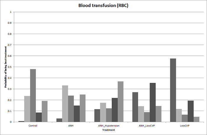
Probability of best treatment: probability of being best, second best, third best, etc. for each treatment for blood transfusion (red blood cells) (cardiopulmonary interventions). A probability of more than 90% is a reliable indicator that a treatment is best with regards to the specific outcome. A probability of less than 90% is less reliable. None of the treatments have a 90% probability of being best treatment.
ANH: acute normovolemic haemodilution; CVP: central venous pressure; RBC: red blood cells.
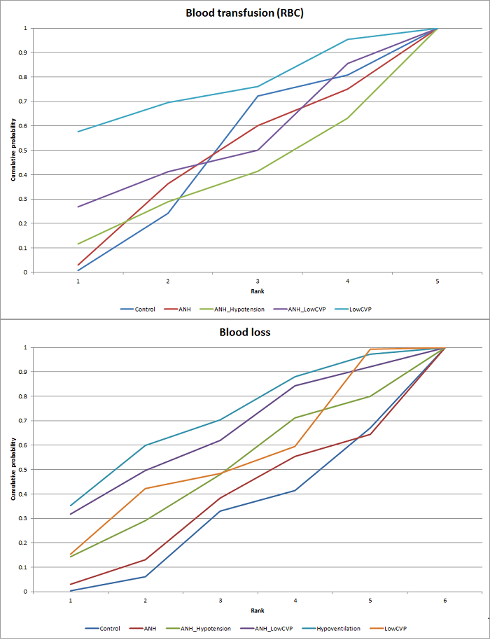
Cumulative probability of being best treatment: cumulative probability of being best for each treatment for cardiopulmonary interventions. Rank 1 indicates the probability that a treatment is best, rank 2 indicates the probability that a treatment is in the two best treatments, rank 3 indicates the probability that a treatment is in the three best treatments, and so on.
ANH: acute normovolemic haemodilution; CVP: central venous pressure; RBC: red blood cells.
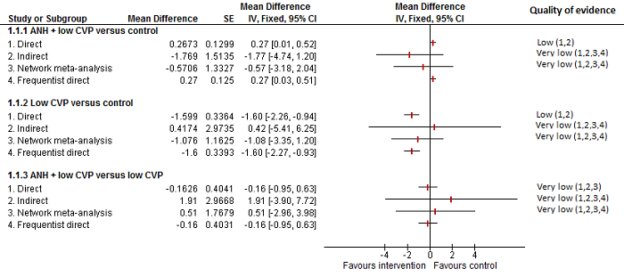
Cardiopulmonary intervention: blood transfusion (red blood cells)
Forest plot of the comparisons in which direct and indirect estimates were available. The mean effect is in opposite directions in the indirect estimate and the direct estimates, thus suggesting that there may be discrepancies between direct and indirect estimates. Direct evidence appears to be preferable over indirect evidence and network meta‐analysis based on the quality of evidence.
1 Risk of bias was unclear or high in the trial(s) (downgraded by 1 point).
2 Sample size was low (downgraded by 1 point).
3Confidence intervals spanned no effect and clinically significant effect (downgraded by 1 point).
4There was substantial or considerable heterogeneity (downgraded by 2 points).

Probability of best treatment: probability of being best, second best, third best, etc. for each treatment for blood loss (cardiopulmonary interventions). A probability of more than 90% is a reliable indicator that a treatment is best with regards to the specific outcome. A probability of less than 90% is less reliable. None of the treatments have a 90% probability of being best treatment.
ANH: acute normovolemic haemodilution; CVP: central venous pressure.
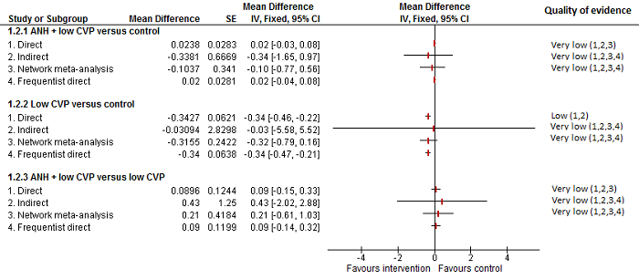
Cardiopulmonary intervention: blood loss
Forest plot of the comparisons in which direct and indirect estimates were available. There does not appear to be any discrepancy between the direct and indirect estimates, although the indirect estimates have wide credible intervals.
Direct evidence appears to be preferable over indirect evidence and network meta‐analysis based on the quality of evidence.
ANH: acute normovolemic haemodilution; CVP: central venous pressure.
1Risk of bias was unclear or high in the trial(s) (downgraded by 1 point).
2Sample size was low (downgraded by 1 point).
3Confidence intervals spanned no effect and clinically significant effect (downgraded by 1 point).
4There was substantial or considerable heterogeneity (downgraded by 2 points).

The network plot showing the comparisons in the trials included in the comparison of methods for parenchymal transection in which network meta‐analysis was performed. The size of the node (circle) provides a measure of the number of trials in which the particular treatment was included as one of the arms. The thickness of the line provides a measure of the number of direct comparisons between two nodes (treatments).
CUSA: cavitron ultrsonic surgical aspirator; RFDS: radiofrequency dissecting sealer.
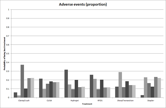
Probability of best treatment: probability of being best, second best, third best, etc. for each treatment for adverse events (proportion) (parenchymal transection methods). A probability of more than 90% is a reliable indicator that a treatment is best with regards to the specific outcome. A probability of less than 90% is less reliable. None of the treatments have a 90% probability of being best treatment.
CUSA: cavitron ultrsonic surgical aspirator; RFDS: radiofrequency dissecting sealer.
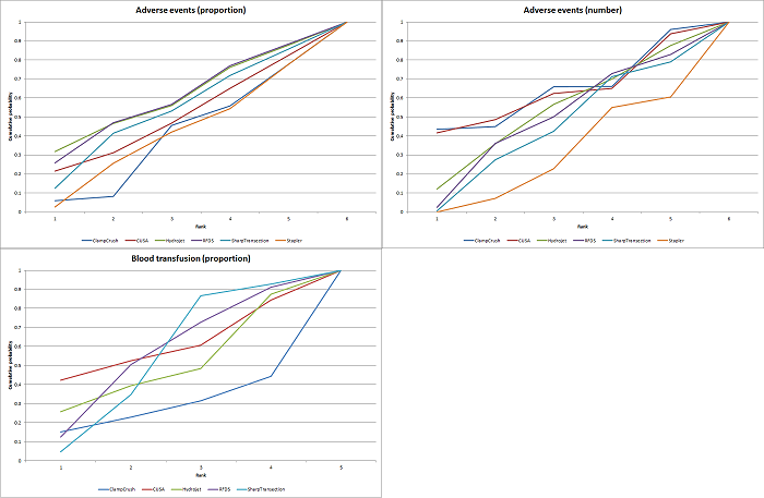
Cumulative probability of being best treatment: cumulative probability of being best for each treatment for parenchymal transection methods. Rank 1 indicates the probability that a treatment is best, rank 2 indicates the probability that a treatment is in the two best treatments, rank 3 indicates the probability that a treatment is in the three best treatments, and so on.
CUSA: cavitron ultrsonic surgical aspirator; RFDS: radiofrequency dissecting sealer.

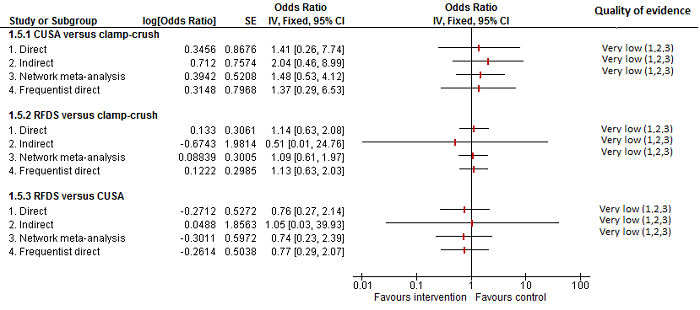
Parenchymal transection: adverse events (proportion)
Forest plot of the comparisons in which direct and indirect estimates were available. There does not appear to be any discrepancy between the direct and indirect estimates, although the indirect estimates have wide credible intervals.
Direct evidence appears to be preferable over indirect evidence and network meta‐analysis based on the quality of evidence.
CUSA: cavitron ultrsonic surgical aspirator; RFDS: radiofrequency dissecting sealer.
1Risk of bias was unclear or high in the trial(s) (downgraded by 1 point).
2Sample size was low (downgraded by 1 point).
3Confidence intervals spanned no effect and clinically significant effect (downgraded by 1 point).
4There was substantial or considerable heterogeneity (downgraded by 2 points).

Probability of best treatment: probability of being best, second best, third best, etc. for each treatment for adverse events (number) (parenchymal transection methods). A probability of more than 90% is a reliable indicator that a treatment is best with regards to the specific outcome. A probability of less than 90% is less reliable. None of the treatments have a 90% probability of being best treatment.
CUSA: cavitron ultrsonic surgical aspirator; RFDS: radiofrequency dissecting sealer.

Parenchymal transection: adverse events (number)
Forest plot of the comparisons in which direct and indirect estimates were available. There does not appear to be any discrepancy between the direct and indirect estimates.
Direct evidence appears to be preferable over indirect evidence and network meta‐analysis based on the quality of evidence.
CUSA: cavitron ultrsonic surgical aspirator; RFDS: radiofrequency dissecting sealer.
1Risk of bias was unclear or high in the trial(s) (downgraded by 1 point).
2Sample size was low (downgraded by 1 point).
3Confidence intervals spanned no effect and clinically significant effect (downgraded by 1 point).

Probability of best treatment: probability of being best, second best, third best, etc. for each treatment for blood transfusion (proportion) (parenchymal transection methods). A probability of more than 90% is a reliable indicator that a treatment is best with regards to the specific outcome. A probability of less than 90% is less reliable. None of the treatments have a 90% probability of being best treatment.
CUSA: cavitron ultrsonic surgical aspirator; RFDS: radiofrequency dissecting sealer.
Parenchymal transection:blood transfusion (proportion)
Forest plot of the comparisons in which direct and indirect estimates were available. There does not appear to be any discrepancy between the direct and indirect estimates, although the indirect estimates have wide credible intervals for some comparisons. There was little apparent difference in the quality of evidence between direct, indirect estimates, and network meta‐analysis; so, we could not choose one estimate over the others based on the quality of evidence.
CUSA: cavitron ultrsonic surgical aspirator; RFDS: radiofrequency dissecting sealer.
1Risk of bias was unclear or high in the trial(s) (downgraded by 1 point).
2Sample size was low (downgraded by 1 point).
3Confidence intervals spanned no effect and clinically significant effect (downgraded by 1 point).

The network plot showing the comparisons in the trials included in the comparison of methods for vascular occlusion in which network meta‐analysis was performed. The size of the node (circle) provides a measure of the number of trials in which the particular treatment was included as one of the arms. The thickness of the line provides a measure of the number of direct comparisons between two nodes (treatments).
Con: continuous; Int: intermittent; HVE: hepatic vascular exclusion; PTC: portal triad clamping; RBC: red blood cells.

Probability of best treatment: probability of being best, second best, third best, etc. for each treatment for serious adverse events (proportion) (vascular occlusion methods). A probability of more than 90% is a reliable indicator that a treatment is best with regards to the specific outcome. A probability of less than 90% is less reliable. None of the treatments have a 90% probability of being best treatment.
Con: continuous; Int: intermittent; HVE: hepatic vascular exclusion; PTC: portal triad clamping.

Cumulative probability of being best treatment: cumulative probability of being best for each treatment for vascular occlusion methods. Rank 1 indicates the probability that a treatment is best, rank 2 indicates the probability that a treatment is in the two best treatments, rank 3 indicates the probability that a treatment is in the three best treatments, and so on.
Con: continuous; Int: intermittent; HVE:hepatic vascular exclusion; PTC: portal triad clamping.
Methods of vascular occlusion: serious adverse events (proportion)
Forest plot of the comparisons in which direct and indirect estimates were available. Although there is overlap of confidence intervals, the mean indirect estimate seems to be quite different from the direct estimate (sometimes, suggesting an opposite effect), thus suggesting that there may be discrepancies between direct and indirect estimates.
There was little apparent difference in the quality of evidence between direct, indirect estimates, and network meta‐analysis; so, we could not choose one estimate over the others based on the quality of evidence.
1Risk of bias was unclear or high in the trial(s) (downgraded by 1 point).
2Sample size was low (downgraded by 1 point).
3Confidence intervals spanned no effect and clinically significant effect (downgraded by 1 point).
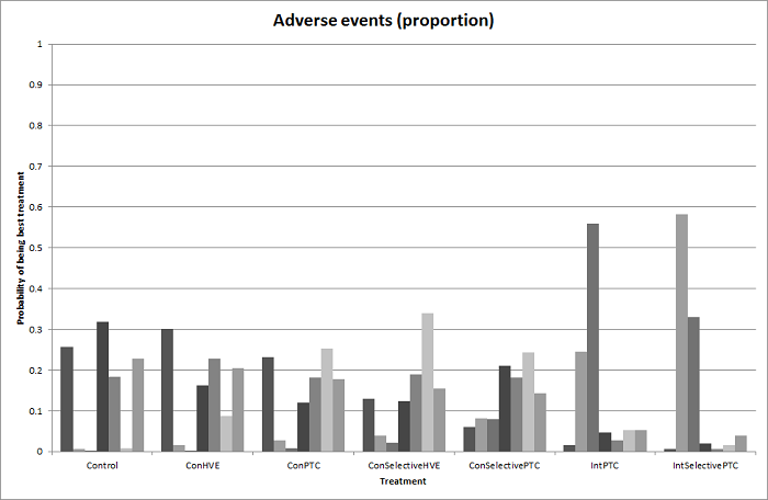
Probability of best treatment: probability of being best, second best, third best, etc. for each treatment for adverse events (proportion) (vascular occlusion methods). A probability of more than 90% is a reliable indicator that a treatment is best with regards to the specific outcome. A probability of less than 90% is less reliable. None of the treatments have a 90% probability of being best treatment.
Con: continuous; Int: intermittent; HVE: hepatic vascular exclusion; PTC: portal triad clamping.

Methods of vascular occlusion: adverse events (proportion)
Forest plot of the comparisons in which direct and indirect estimates were available. There does not appear to be any discrepancies between direct and indirect estimates. Direct evidence appears to be preferable over indirect evidence and network meta‐analysis based on the quality of evidence.
1Risk of bias was unclear or high in the trial(s) (downgraded by 1 point).
2Sample size was low (downgraded by 1 point).
3Confidence intervals spanned no effect and clinically significant effect (downgraded by 1 point).
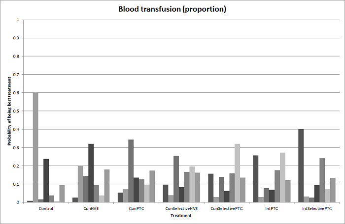
Probability of best treatment: probability of being best, second best, third best, etc. for each treatment for blood transfusion (proportion) (vascular occlusion methods). A probability of more than 90% is a reliable indicator that a treatment is best with regards to the specific outcome. A probability of less than 90% is less reliable. None of the treatments have a 90% probability of being best treatment.
Con: continuous; Int: intermittent; HVE: hepatic vascular exclusion; PTC: portal triad clamping.

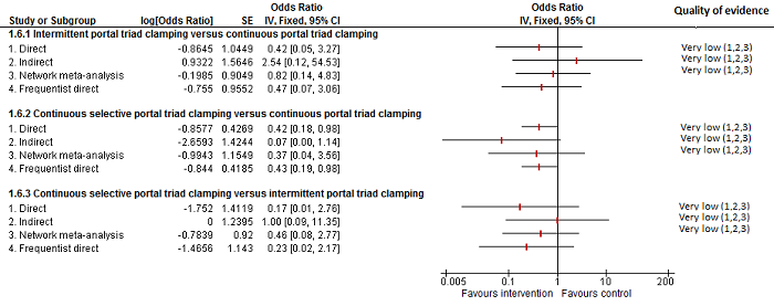
Methods of vascular occlusion: blood transfusion (proportion)
Forest plot of the comparisons in which direct and indirect estimates were available. Although the confidence intervals overlap, there appear to be some discrepancies between direct and indirect estimates for continuous portal triad clamping versus control, intermittent portal triad clamping versus control, and intermittent portal triad clamping versus continuous portal triad clamping. Direct evidence appears to be preferable over indirect evidence and network meta‐analysis based on the quality of evidence.
1Risk of bias was unclear or high in the trial(s) (downgraded by 1 point).
2Sample size was low (downgraded by 1 point).
3Confidence intervals spanned no effect and clinically significant effect (downgraded by 1 point).
4There was substantial or considerable heterogeneity (downgraded by 2 points).

Probability of best treatment: probability of being best, second best, third best, etc. for each treatment for blood transfusion (red blood cells) (vascular occlusion methods). A probability of more than 90% is a reliable indicator that a treatment is best with regards to the specific outcome. A probability of less than 90% is less reliable. Intermittent selective portal triad clamping has about 90% probability of being best treatment. However, other random and systematic errors make this finding unreliable.
Con: continuous; Int: intermittent; HVE: hepatic vascular exclusion; PTC: portal triad clamping.

Methods of vascular occlusion:blood transfusion (red blood cells)
Forest plot of the comparisons in which direct and indirect estimates were available. There do not appear to be any discrepancies between direct and indirect estimates, although the credible intervals are different (the direct evidence had narrower credible intervals in four of the five comparisons above) resulting in the differences in the comparisons in which there was evidence for difference. Direct evidence appears to be preferable over indirect evidence and network meta‐analysis based on the quality of evidence for the comparison 'continuous selective portal triad clamping versus continuous portal triad clamping'. Indirect evidence and network meta‐analysis appear to be preferable over direct evidence for the comparison 'continuous portal triad clamping versus control'. Direct evidence and network meta‐analysis appear to be preferable over indirect evidence for the comparison 'intermittent portal triad clamping versus control'. There was little apparent difference in the quality of evidence between direct, indirect estimates, and network meta‐analysis; so, we could not choose one estimate over the others based on the quality of evidence.
1Risk of bias was unclear or high in the trial(s) (downgraded by 1 point).
2Sample size was low (downgraded by 1 point).
3Confidence intervals spanned no effect and clinically significant effect (downgraded by 1 point).

Probability of best treatment: probability of being best, second best, third best, etc. for each treatment for blood loss (vascular occlusion methods). A probability of more than 90% is a reliable indicator that a treatment is best with regards to the specific outcome. A probability of less than 90% is less reliable. None of the treatments have a 90% probability of being best treatment.
Con: continuous; Int: intermittent; HVE: hepatic vascular exclusion; PTC: portal triad clamping.

Methods of vascular occlusion:blood loss
Forest plot of the comparisons in which direct and indirect estimates were available. There does not appear to be any discrepancies between direct and indirect estimates, although the credible intervals are different (the direct evidence had narrower credible intervals in three of the five comparisons above). Direct evidence appears to be preferable over indirect evidence and network meta‐analysis based on the quality of evidence.
1Risk of bias was unclear or high in the trial(s) (downgraded by 1 point).
2 Sample size was low (downgraded by 1 point).
3Confidence intervals spanned no effect and clinically significant effect (downgraded by 1 point).Ç
4There was substantial or considerable heterogeneity (downgraded by 2 points).

Funnel plot of blood transfusion (proportion): The funnel plot shows funnel plot asymmetry (i.e. some trials with large variance with large effects favouring one treatment were not matched by other trials with similarly large variance with large effects favouring the other treatment). This may be evidence of reporting bias or could be because of heterogeneity between the studies.

Funnel plot of blood transfusion (red blood cells): The funnel plot shows funnel plot asymmetry (i.e. some trials with large variance with large effects favouring one treatment were not matched by other trials with similarly large variance with large effects favouring the other treatment). This may be evidence of reporting bias or could be because of heterogeneity between the studies.

Funnel plot of blood loss: The funnel plot shows funnel plot asymmetry (i.e. some trials with large variance with large effects favouring one treatment were not matched by other trials with similarly large variance with large effects favouring the other treatment). This may be evidence of reporting bias or could be because of heterogeneity between the studies.

Comparison 1 Anterior approach vs conventional approach, Outcome 1 Mortality (perioperative).

Comparison 1 Anterior approach vs conventional approach, Outcome 2 Serious adverse events (proportion).

Comparison 1 Anterior approach vs conventional approach, Outcome 3 Adverse events (proportion).
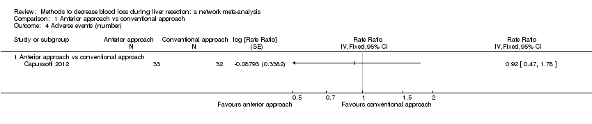
Comparison 1 Anterior approach vs conventional approach, Outcome 4 Adverse events (number).
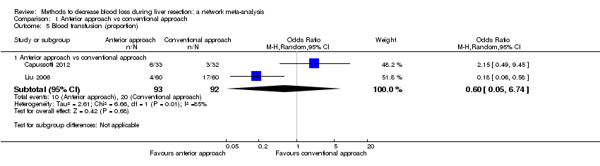
Comparison 1 Anterior approach vs conventional approach, Outcome 5 Blood transfusion (proportion).
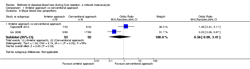
Comparison 1 Anterior approach vs conventional approach, Outcome 6 Major blood loss (proportion).

Comparison 2 Autologous blood donation vs control, Outcome 1 Adverse events (proportion).

Comparison 2 Autologous blood donation vs control, Outcome 2 Blood transfusion (proportion).
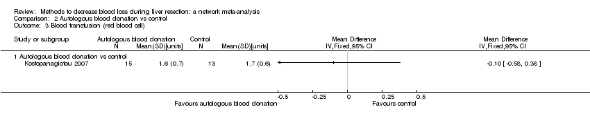
Comparison 2 Autologous blood donation vs control, Outcome 3 Blood transfusion (red blood cell).

Comparison 2 Autologous blood donation vs control, Outcome 4 Blood loss.

Comparison 2 Autologous blood donation vs control, Outcome 5 Major blood loss (proportion).

Comparison 2 Autologous blood donation vs control, Outcome 6 Total hospital stay.

Comparison 2 Autologous blood donation vs control, Outcome 7 Operating time.

Comparison 3 Cardiopulmonary interventions, Outcome 1 Mortality (perioperative).

Comparison 3 Cardiopulmonary interventions, Outcome 2 Serious adverse events (proportion).

Comparison 3 Cardiopulmonary interventions, Outcome 3 Serious adverse events (number).
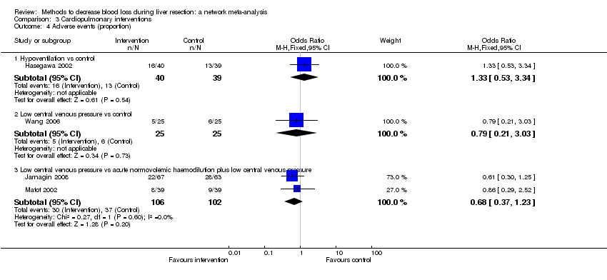
Comparison 3 Cardiopulmonary interventions, Outcome 4 Adverse events (proportion).

Comparison 3 Cardiopulmonary interventions, Outcome 5 Adverse events (number).

Comparison 3 Cardiopulmonary interventions, Outcome 6 Blood transfusion (proportion).

Comparison 3 Cardiopulmonary interventions, Outcome 7 Blood transfusion (red blood cell).
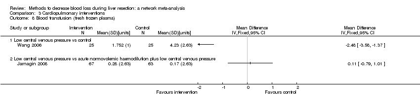
Comparison 3 Cardiopulmonary interventions, Outcome 8 Blood transfusion (fresh frozen plasma).
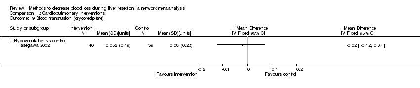
Comparison 3 Cardiopulmonary interventions, Outcome 9 Blood transfusion (cryoprecipitate).
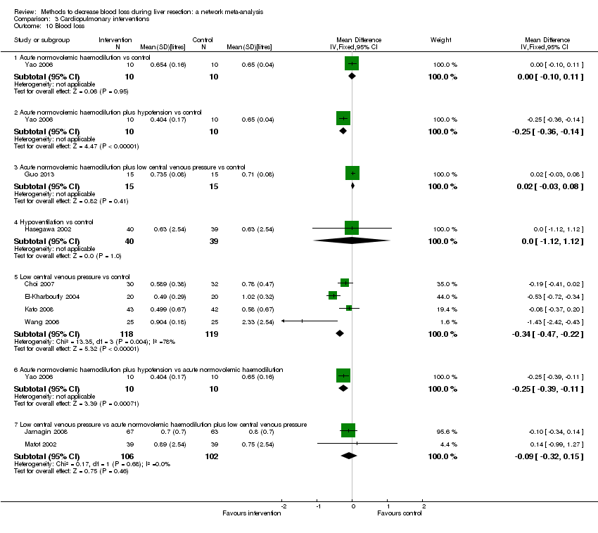
Comparison 3 Cardiopulmonary interventions, Outcome 10 Blood loss.
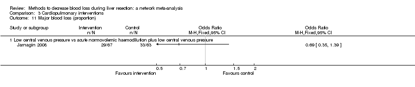
Comparison 3 Cardiopulmonary interventions, Outcome 11 Major blood loss (proportion).

Comparison 3 Cardiopulmonary interventions, Outcome 12 Hospital stay.
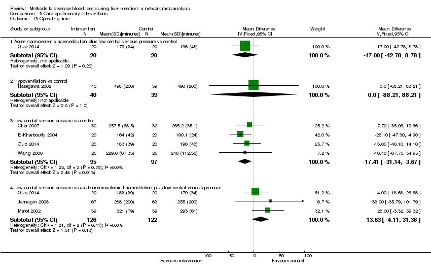
Comparison 3 Cardiopulmonary interventions, Outcome 13 Operating time.

Comparison 4 Methods of parenchymal transection, Outcome 1 Mortality (perioperative).
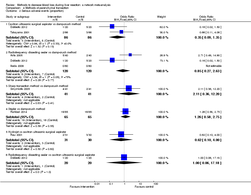
Comparison 4 Methods of parenchymal transection, Outcome 2 Serious adverse events (proportion).

Comparison 4 Methods of parenchymal transection, Outcome 3 Serious adverse events (number).

Comparison 4 Methods of parenchymal transection, Outcome 4 Adverse events (proportion).

Comparison 4 Methods of parenchymal transection, Outcome 5 Adverse events (number).

Comparison 4 Methods of parenchymal transection, Outcome 6 Blood transfusion (proportion).

Comparison 4 Methods of parenchymal transection, Outcome 7 Blood transfusion (red blood cell).

Comparison 4 Methods of parenchymal transection, Outcome 8 Blood transfusion (fresh frozen plasma).
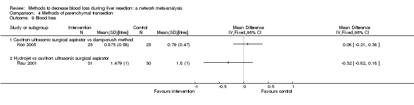
Comparison 4 Methods of parenchymal transection, Outcome 9 Blood loss.

Comparison 4 Methods of parenchymal transection, Outcome 10 Operating time.
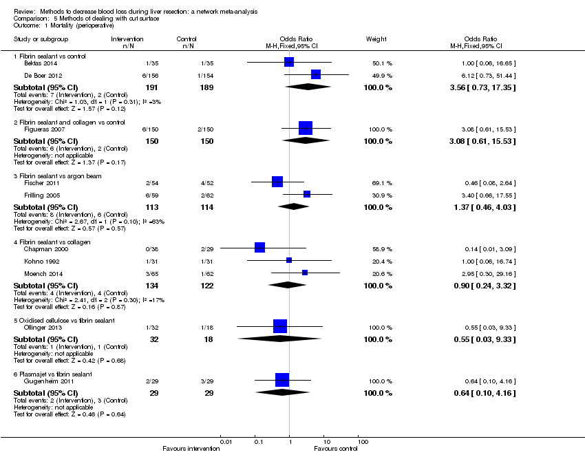
Comparison 5 Methods of dealing with cut surface, Outcome 1 Mortality (perioperative).

Comparison 5 Methods of dealing with cut surface, Outcome 2 Serious adverse events (proportion).

Comparison 5 Methods of dealing with cut surface, Outcome 3 Serious adverse events (number).

Comparison 5 Methods of dealing with cut surface, Outcome 4 Adverse events (proportion).

Comparison 5 Methods of dealing with cut surface, Outcome 5 Adverse events (number).
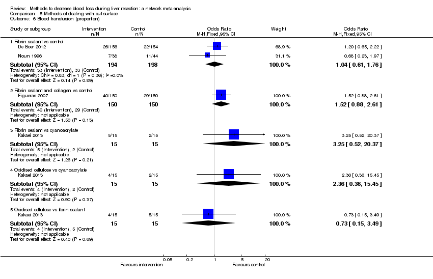
Comparison 5 Methods of dealing with cut surface, Outcome 6 Blood transfusion (proportion).
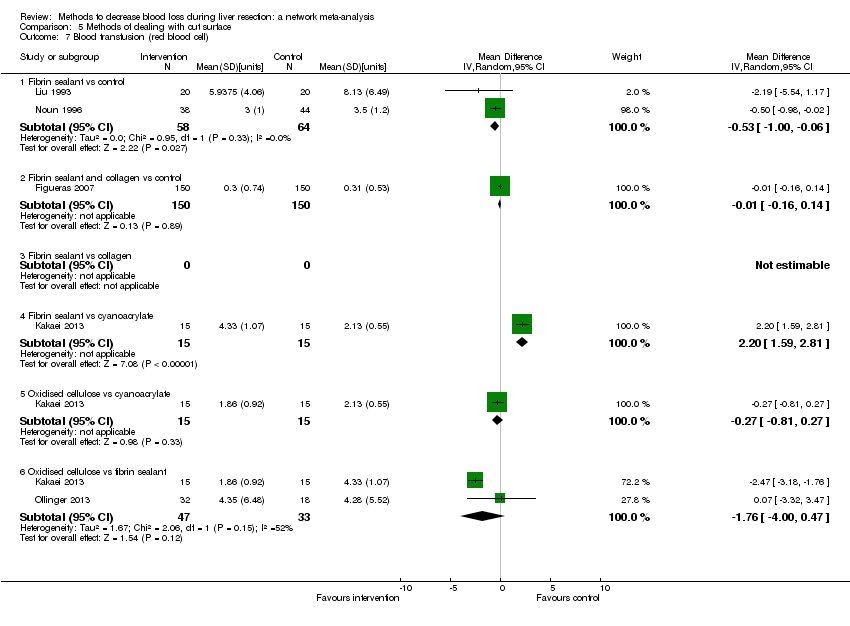
Comparison 5 Methods of dealing with cut surface, Outcome 7 Blood transfusion (red blood cell).

Comparison 5 Methods of dealing with cut surface, Outcome 8 Blood transfusion (fresh frozen plasma).

Comparison 5 Methods of dealing with cut surface, Outcome 9 Blood loss.

Comparison 5 Methods of dealing with cut surface, Outcome 10 Total hospital stay.
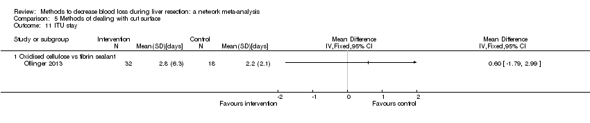
Comparison 5 Methods of dealing with cut surface, Outcome 11 ITU stay.

Comparison 5 Methods of dealing with cut surface, Outcome 12 Operating time.

Comparison 6 Methods of vascular occlusion, Outcome 1 Mortality (perioperative).

Comparison 6 Methods of vascular occlusion, Outcome 2 Serious adverse events (proportion).
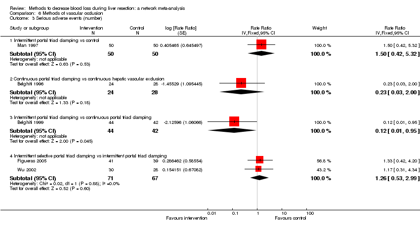
Comparison 6 Methods of vascular occlusion, Outcome 3 Serious adverse events (number).
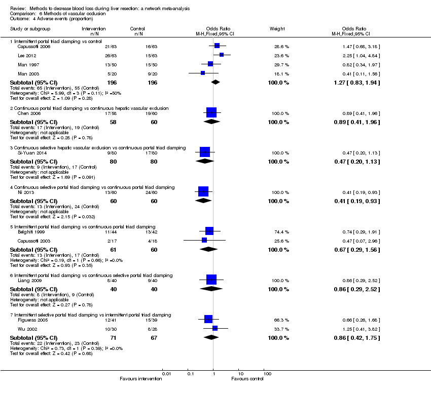
Comparison 6 Methods of vascular occlusion, Outcome 4 Adverse events (proportion).

Comparison 6 Methods of vascular occlusion, Outcome 5 Adverse events (number).

Comparison 6 Methods of vascular occlusion, Outcome 6 Blood transfusion (proportion).
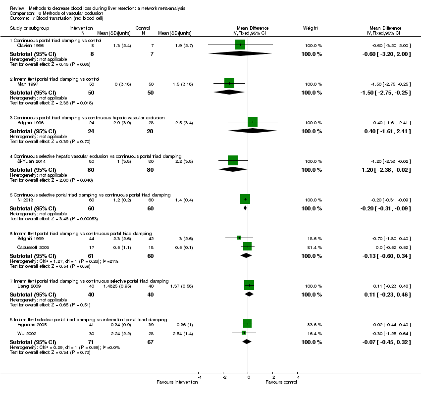
Comparison 6 Methods of vascular occlusion, Outcome 7 Blood transfusion (red blood cell).
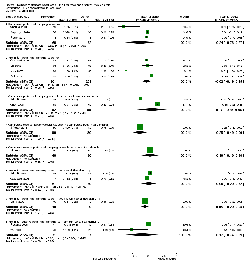
Comparison 6 Methods of vascular occlusion, Outcome 8 Blood loss.

Comparison 6 Methods of vascular occlusion, Outcome 9 Major blood loss (proportion).

Comparison 6 Methods of vascular occlusion, Outcome 10 Total hospital stay.

Comparison 6 Methods of vascular occlusion, Outcome 11 ITU stay.

Comparison 6 Methods of vascular occlusion, Outcome 12 Operating time.

Comparison 7 Pharmacological interventions, Outcome 1 Mortality (perioperative).

Comparison 7 Pharmacological interventions, Outcome 2 Serious adverse events (proportion).
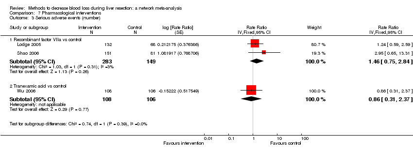
Comparison 7 Pharmacological interventions, Outcome 3 Serious adverse events (number).

Comparison 7 Pharmacological interventions, Outcome 4 Adverse events (proportion).
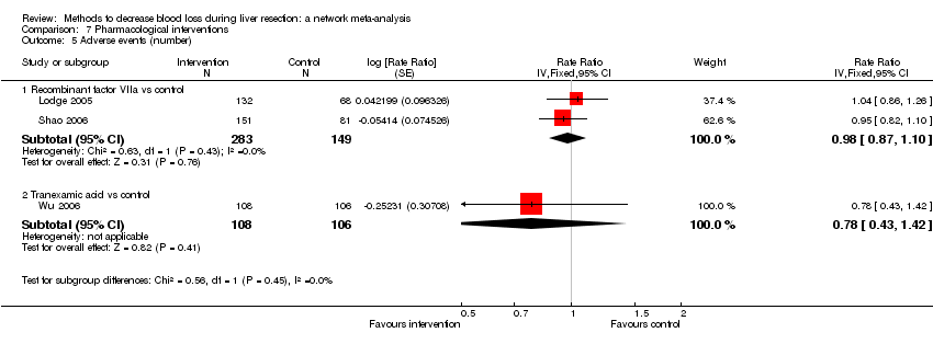
Comparison 7 Pharmacological interventions, Outcome 5 Adverse events (number).
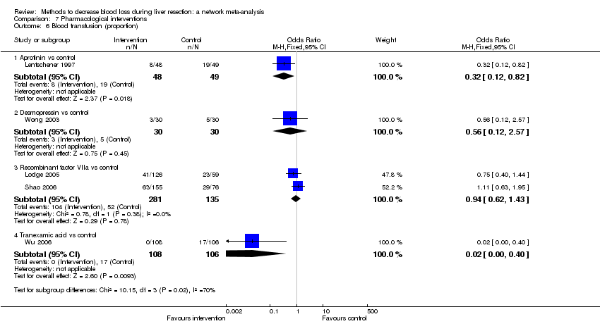
Comparison 7 Pharmacological interventions, Outcome 6 Blood transfusion (proportion).

Comparison 7 Pharmacological interventions, Outcome 7 Blood transfusion (fresh frozen plasma).

Comparison 7 Pharmacological interventions, Outcome 8 Blood loss.

Comparison 7 Pharmacological interventions, Outcome 9 Hospital stay.

Comparison 7 Pharmacological interventions, Outcome 10 Operating time.
| Methods to decrease blood loss during liver resection: a network meta‐analysis. Primary outcomes | |||||||
| Patient or population: people undergoing liver resection Settings: secondary or tertiary setting Intervention and control: various treatments Follow‐up: until discharge or 1 month (except for mortality (long‐term follow‐up) which was reported at 1 year | |||||||
| Outcomes | Anterior approach versus conventional approach | Autologous blood donation versus control | Cardiopulmonary interventions | Methods of parenchymal transection | Methods of dealing with cut surface | Methods of vascular occlusion | Pharmacological interventions |
| Treatments The first treatment listed is the control. The remaining are interventions. |
|
|
|
|
|
|
|
| Link for detailed 'Summary of Findings tables' | |||||||
| Mortality (perioperative) | There was no evidence of differences in perioperative mortality between the 2 groups. Quality of evidence = very low1,2,3. | There was no evidence of differences in perioperative mortality between the two groups. Quality of evidence = very low1,2,3. | There was no evidence of differences in perioperative mortality for any of the comparisons. Quality of evidence = very low1,2,3. | There was no evidence of differences in perioperative mortality for any of the comparisons. Quality of evidence = very low1,2,3. | There was no evidence of differences in perioperative mortality for any of the comparisons Quality of evidence = very low1,2,3. | There was no evidence of differences in perioperative mortality for any of the comparisons. Quality of evidence = very low1,2,3. | There was no evidence of differences in perioperative mortality for any of the comparisons. Quality of evidence = very low1,2,3. |
| Mortality (longest follow‐up) | None of the trials reported this outcome. | There was no evidence of differences in mortality at 1 year between the 2 groups. Quality of evidence = very low)1,2,3. | None of the trials reported this outcome. | None of the trials reported this outcome. | None of the trials reported this outcome. | None of the trials reported this outcome. | None of the trials reported this outcome. |
| Serious adverse events (proportion) | There was no evidence of differences in the proportion of participants experiencing serious adverse events between the 2 groups. Quality of evidence = very low1,2,3. | None of the trials reported this outcome. | There was no evidence of differences in the proportion of participants experiencing serious adverse events (for any of the comparisons Quality of evidence = very low1,2,3. | There was no evidence of differences in the proportion of participants experiencing serious adverse events for any of the comparisons Quality of evidence = very low1,2,3. | There was no evidence of differences in the proportion of participants experiencing serious adverse events for any of the comparisons Quality of evidence = very low1,2,3. | The proportion of participants experiencing serious adverse eventsa was lower in continuous selective portal triad clamping than continuous portal triad clamping
There was no evidence of differences in other comparisons. Quality of evidence = very low1,2,3 | There was no evidence of differences in the proportion of participants experiencing serious adverse events for any of the comparisons Quality of evidence = very low1,2,3. |
| Serious adverse events (number) | None of the trials reported this outcome. | None of the trials reported this outcome. | There was no evidence of differences in the number of serious adverse events for any of the comparisons Quality of evidence = very low1,2,3. | The number of serious adverse events was higher in radiofrequency dissecting sealer than clamp‐crush method.
There was no evidence of differences in other comparisons. Quality of evidence = very low1,2,3. | The number of serious adverse events was higher in fibrin sealant than argon beam.
There was no evidence of differences in other comparisons. Quality of evidence = very low1,2,3. | The number of serious adverse events was lower in intermittent portal triad clamping than continuous portal triad clamping.
There was no evidence of differences in other comparisons Quality of evidence = very low1,2,3. | There was no evidence of differences in the number of serious adverse events for any of the comparisons Quality of evidence = very low1,2,3. |
| Health‐related quality of life | None of the trials reported this outcome. | None of the trials reported this outcome. | None of the trials reported this outcome at any time point. | None of the trials reported this outcome at any time point. | None of the trials reported this outcome at any time point. | None of the trials reported this outcome at any time point. | None of the trials reported this outcome at any time point. |
| CrI: credible intervals; OR: odds ratio. | |||||||
| GRADE Working Group grades of evidence | |||||||
| 1 Risk of bias was unclear or high in the trial(s) (downgraded by 1 point). | |||||||
| Outcomes | Illustrative comparative risks* (95% CrI) | Relative effect (95% CrI) | No of participants | Quality of the evidence | |
| Assumed risk | Corresponding risk | ||||
| Control | Intervention | ||||
| Mortality (perioperative) | 76 per 1000 | 19 per 1000 | OR 0.23 | 185 | ⊕⊝⊝⊝ |
| Mortality (longest follow‐up) | None of the trials reported this outcome. | ||||
| Serious adverse events (proportion) | 125 per 1000 | 154 per 1000 | OR 1.27 | 65 | ⊕⊝⊝⊝ |
| Serious adverse events (number) | None of the trials reported this outcome. | ||||
| Health‐related quality of life (30 days, 3 months) | None of the trials reported this outcome. | ||||
| Health‐related quality of life (maximal follow‐up) | None of the trials reported this outcome. | ||||
| *The basis for the assumed risk is the mean control group proportion. The corresponding risk (and its 95% credible interval) is based on the assumed risk in the comparison group and the relative effect of the intervention (and its 95% CrI). Network meta‐analysis was not performed for any of the outcomes since there were only two treatments. CrI: credible intervals; OR: odds ratio. | |||||
| GRADE Working Group grades of evidence | |||||
| 1 Risk of bias was unclear or high in the trial(s) (downgraded by 1 point). | |||||
| Outcomes | Illustrative comparative risks* (95% CrI) | Relative effect (95% CrI) | No of participants | Quality of the evidence | |
| Assumed risk | Corresponding risk | ||||
| Control | Intervention | ||||
| Mortality (perioperative) | There was no mortality in either group. | 28 (1 study) | ⊕⊝⊝⊝ Very low1,2,3 | ||
| Mortality (longest follow‐up): reported at 1 year | There was no mortality in either group. | 28 (1 study) | ⊕⊝⊝⊝ Very low1,2,3 | ||
| Serious adverse events (proportion) | None of the trials reported this outcome. | ||||
| Serious adverse events (number) | None of the trials reported this outcome. | ||||
| Health‐related quality of life (30 days, 3 months) | None of the trials reported this outcome. | ||||
| Health‐related quality of life (longest follow‐up) | None of the trials reported this outcome. | ||||
| *The basis for the assumed risk is the mean control group proportion. The corresponding risk (and its 95% credible interval) is based on the assumed risk in the comparison group and the relative effect of the intervention (and its 95% CrI). Network meta‐analysis was not performed for any of the outcomes since there were only two treatments. CrI: credible intervals; OR: odds ratio | |||||
| GRADE Working Group grades of evidence | |||||
| 1 Risk of bias was unclear or high in the trial(s) (downgraded by 1 point). | |||||
| Outcomes | Illustrative comparative risks* (95% CrI) | Relative effect (95% CrI) | No of participants | Quality of the evidence | |
| Assumed risk | Corresponding risk | ||||
| Control | Intervention | ||||
| Mortality (perioperative) | |||||
| Hypoventilation vs control | There was no mortality in either group. | 79 (1 study) | ⊕⊝⊝⊝ Very low1,2,3 | ||
| Low central venous pressure vs control | There was no mortality in either group. | 85 (1 study) | ⊕⊝⊝⊝ Very low1,2,3 | ||
| Mortality (longest follow‐up) | None of the trials reported this outcome. | ||||
| Serious adverse events (proportion) | |||||
| Hypoventilation vs control | 26 per 1000 | 60 per 1000 (5 to 679) | OR 2.41 (0.18 to 80.4) | 79 (1 study) | ⊕⊝⊝⊝ Very low1,2,3 |
| Low central venous pressure vs acute normovolemic haemodilution plus low CVP | 302 per 1000 | 284 per 1000 (157 to 460) | OR 0.92 (0.43 to 1.97) | 63 (1 study) | ⊕⊝⊝⊝ Very low1,2,3 |
| Serious adverse events (number) | |||||
| Low central venous pressure vs control | 100 per 1000 | 0 per 1000 (0 to 2) | Rate ratio 0.00 (0 to 0.02) | 42 (1 study) | ⊕⊝⊝⊝ Very lowa,b,c |
| Low central venous pressure vs acute normovolemic haemodilution plus low central venous pressure | 103 per 1000 | 77 per 1000 (15 to 287) | Rate ratio 0.73 (0.13 to 3.53) | 78 (1 study) | ⊕⊝⊝⊝ Very lowa,b,c |
| Health‐related quality of life (30 days, 3 months) | None of the trials reported this outcome. | ||||
| Health‐related quality of life (longest follow‐up) | None of the trials reported this outcome. | ||||
| *The basis for the assumed risk is the mean control group proportion. The corresponding risk (and its 95% credible interval) is based on the assumed risk in the comparison group and the relative effect of the intervention (and its 95% CrI). Network meta‐analysis was not performed for any of the outcomes because of the lack of availability of direct and indirect comparisons in the network. CrI: credible intervals; OR: odds ratio. | |||||
| GRADE Working Group grades of evidence | |||||
| 1aRisk of bias was unclear or high in the trial(s) (downgraded by 1 point). | |||||
| Outcomes | Illustrative comparative risks* (95% CrI) | Relative effect (95% CrI) | No of participants | Quality of the evidence | |
| Assumed risk | Corresponding risk | ||||
| Control | Intervention | ||||
| Mortality (perioperative) | |||||
| CUSA vs clamp‐crush method | 23 per 1000 | 6 per 1000 (0 to 54) | OR 0.24 (0.01 to 2.41) | 172 (2 studies) | ⊕⊝⊝⊝ Very low1,2,3 |
| Radiofrequency dissecting sealer vs clamp‐crush method | 10 per 1000 | 16 per 1000 (4 to 65) | OR 1.60 (0.43 to 6.7) | 390 (5 studies) | ⊕⊝⊝⊝ Very low1,2,3 |
| Sharp transection method vs clamp‐crush method | There was no mortality in either group. | 82 (1 study) | ⊕⊝⊝⊝ Very low1,2,3 | ||
| Stapler vs clamp‐crush method | 31 per 1000 | 67 per 1000 (12 to 375) | OR 2.26 (0.39 to 18.93) | 130 (1 study) | ⊕⊝⊝⊝ Very low1,2,3 |
| Hydrojet vs CUSA | 55 per 1000 | 54 per 1000 (9 to 258) | OR 0.98 (0.16 to 6.04) | 111 (2 studies) | ⊕⊝⊝⊝ Very low1,2,3 |
| Radiofrequency dissecting sealer vs CUSA | 44 per 1000 | 28 per 1000 (3 to 166) | OR 0.61 (0.07 to 4.28) | 90 (2 studies) | ⊕⊝⊝⊝ Very low1,2,3 |
| Stapler vs CUSA | There was no mortality in either group. | 79 (1 study) | ⊕⊝⊝⊝ Very low1,2,3 | ||
| Radiofrequency dissecting sealer vs hydrojet | 80 per 1000 | 9 per 1000 (0 to 145) | OR 0.10 (0 to 1.95) | 50 (1 study) | ⊕⊝⊝⊝ Very low1,2,3 |
| Mortality (longest follow‐up) | None of the trials reported this outcome. | ||||
| Serious adverse events (proportion) | |||||
| CUSA vs clamp‐crush method | 93 per 1000 | 31 per 1000 (6 to 110) | OR 0.31 (0.06 to 1.2) | 172 (2 studies) | ⊕⊝⊝⊝ Very low1,2,3 |
| Radiofrequency dissecting sealer vs clamp‐crush method | 58 per 1000 | 49 per 1000 (15 to 145) | OR 0.83 (0.24 to 2.74) | 240 (3 studies) | ⊕⊝⊝⊝ Very low1,2,3 |
| Sharp transection method vs clamp‐crush method | 49 per 1000 | 106 per 1000 (20 to 502) | OR 2.31 (0.39 to 19.69) | 82 (1 study) | ⊕⊝⊝⊝ Very low1,2,3 |
| Hydrojet vs CUSA | 100 per 1000 | 124 per 1000 (61 to 238) | OR 1.27 (0.58 to 2.81) | 61 (1 study) | ⊕⊝⊝⊝ Very low1,2,3 |
| Radiofrequency dissecting sealer vs CUSA | 50 per 1000 | 30 per 1000 (3 to 180) | OR 0.58 (0.06 to 4.16) | 40 (1 study) | ⊕⊝⊝⊝ Very low1,2,3 |
| Stapler vs CUSA | 246 per 1000 | 246 per 1000 (6 to 931) | OR 1.00 (0.02 to 41.22) | 130 (1 study) | ⊕⊝⊝⊝ Very low1,2,3 |
| Serious adverse events (number) | |||||
| CUSA vs clamp‐crush method | 45 per 1000 | 29 per 1000 (3 to 166) | Rate ratio 0.63 (0.07 to 4.17) | 132 (1 study) | ⊕⊝⊝⊝ Very low1,2,3 |
| Radiofrequency dissecting sealer vs clamp‐crush method | 61 per 1000 | 190 per 1000 (75 to 474) | Rate ratio 3.64 (1.25 to 13.97) | 130 (2 studies) | ⊕⊕⊝⊝ Low1,2 |
| Hydrojet vs CUSA | 80 per 1000 | 121 per 1000 (20 to 546) | Rate ratio 1.59 (0.24 to 13.83) | 50 (1 study) | ⊕⊝⊝⊝ Very low1,2,3 |
| Radiofrequency dissecting sealer vs CUSA | 80 per 1000 | 121 per 1000 (20 to 546) | Rate ratio 1.59 (0.24 to 13.83) | 50 (1 study) | ⊕⊝⊝⊝ Very low1,2,3 |
| Stapler vs CUSA | 180 per 1000 | 230 per 1000 (109 to 424) | Rate ratio 1.36 (0.56 to 3.36) | 100 (1 study) | ⊕⊝⊝⊝ Very low1,2,3 |
| Radiofrequency dissecting sealer vs hydrojet | 120 per 1000 | 120 per 1000 (23 to 445) | Rate ratio 1.00 (0.17 to 5.88) | 50 (1 study) | ⊕⊝⊝⊝ Very low1,2,3 |
| Health‐related quality of life (30 days, 3 months) | None of the trials reported this outcome. | ||||
| Health‐related quality of life (maximal follow‐up) | None of the trials reported this outcome. | ||||
| *The basis for the assumed risk is the mean control group proportion. The corresponding risk (and its 95% credible interval) is based on the assumed risk in the comparison group and the relative effect of the intervention (and its 95% CrI). Network meta‐analysis was not performed for any of the outcomes because of the lack of availability of direct and indirect comparisons in the network. CrI: credible intervals; CUSA: cavitron ultrasonic surgical aspirator; OR: odds ratio | |||||
| GRADE Working Group grades of evidence | |||||
| 1 Risk of bias was unclear or high in the trial(s) (downgraded by 1 point). | |||||
| Outcomes | Illustrative comparative risks* (95% CrI) | Relative effect (95% CrI) | No of participants | Quality of the evidence | |
| Assumed risk | Corresponding risk | ||||
| Control | Intervention | ||||
| Mortality (perioperative) | |||||
| Fibrin sealant vs control | 11 per 1000 | 41 per 1000 (10 to 253) | OR 4.03 (0.9 to 31.72) | 380 (2 studies) | ⊕⊝⊝⊝ Very low1,2,3 |
| Fibrin sealant and collagen vs control | 13 per 1000 | 45 per 1000 (10 to 268) | OR 3.48 (0.74 to 27.03) | 300 (1 study) | ⊕⊝⊝⊝ Very low1,2,3 |
| Fibrin sealant vs argon beam | 53 per 1000 | 72 per 1000 (25 to 198) | OR 1.39 (0.46 to 4.45) | 227 (2 studies) | ⊕⊝⊝⊝ Very low1,2,3 |
| Fibrin sealant vs collagen | 33 per 1000 | 30 per 1000 (7 to 123) | OR 0.91 (0.2 to 4.14) | 256 (3 studies) | ⊕⊝⊝⊝ Very low1,2,3 |
| Oxidised cellulose vs fibrin sealant | 56 per 1000 | 31 per 1000 (1 to 565) | OR 0.54 (0.01 to 22.09) | 50 (1 study) | ⊕⊝⊝⊝ Very low1,2,3 |
| Plasmajet vs fibrin sealant | 103 per 1000 | 65 per 1000 (7 to 332) | OR 0.60 (0.06 to 4.31) | 58 (1 study) | ⊕⊝⊝⊝ Very low1,2,3 |
| Mortality (longest follow‐up) | None of the trials reported this outcome. | ||||
| Serious adverse events (proportion) | |||||
| Fibrin sealant vs control | 186 per 1000 | 191 per 1000 (128 to 275) | OR 1.03 (0.64 to 1.66) | 457 (3 studies) | ⊕⊝⊝⊝ Very low1,2,3 |
| Fibrin sealant vs argon beam | 269 per 1000 | 183 per 1000 (78 to 360) | OR 0.61 (0.23 to 1.53) | 106 (1 study) | ⊕⊝⊝⊝ Very low1,2,3 |
| Fibrin sealant vs collagen | 258 per 1000 | 356 per 1000 (205 to 547) | OR 1.59 (0.74 to 3.47) | 127 (1 study) | ⊕⊝⊝⊝ Very low1,2,3 |
| Oxidised cellulose vs fibrin sealant | 444 per 1000 | 309 per 1000 (113 to 603) | OR 0.56 (0.16 to 1.9) | 50 (1 study) | ⊕⊝⊝⊝ Very low1,2,3 |
| Plasmajet vs fibrin sealant | 207 per 1000 | 25 per 1000 (0 to 165) | OR 0.10 (0 to 0.76) | 58 (1 study) | ⊕⊝⊝⊝ Very low1,2,3 |
| Serious adverse events (number) | |||||
| Fibrin sealant vs control | 486 per 1000 | 470 per 1000 (307 to 640) | Rate ratio 0.94 (0.47 to 1.88) | 70 (1 study) | ⊕⊝⊝⊝ Very low1,2,3 |
| Fibrin sealant & collagen vs control | 147 per 1000 | 186 per 1000 (116 to 286) | Rate ratio 1.33 (0.76 to 2.33) | 300 (1 study) | ⊕⊝⊝⊝ Very low1,2,3 |
| Fibrin sealant vs argon beam | 65 per 1000 | 249 per 1000 (107 to 547) | Rate ratio 4.81 (1.73 to 17.5) | 121 (1 study) | ⊕⊕⊝⊝ Low1,2 |
| Fibrin sealant vs collagen | 323 per 1000 | 369 per 1000 (266 to 488) | Rate ratio 1.23 (0.76 to 2) | 189 (2 studies) | ⊕⊝⊝⊝ Very low1,2,3 |
| Fibrin sealant vs cyanoacrylate | 67 per 1000 | 67 per 1000 (2 to 733) | Rate ratio 1.01 (0.03 to 38.36) | 30 (1 study) | ⊕⊝⊝⊝ Very low1,2,3 |
| Oxidised cellulose vs cyanoacrylate | 67 per 1000 | 277 per 1000 (46 to 921) | Rate ratio 5.37 (0.67 to 163.2) | 30 (1 study) | ⊕⊝⊝⊝ Very low1,2,3 |
| Oxidised cellulose vs fibrin sealant | 67 per 1000 | 278 per 1000 (46 to 926) | Rate ratio 5.40 (0.67 to 174.86) | 30 (1 study) | ⊕⊝⊝⊝ Very low1,2,3 |
| Health‐related quality of life (30 days, 3 months) | None of the trials reported this outcome. | ||||
| Health‐related quality of life (longest follow‐up) | None of the trials reported this outcome. | ||||
| *The basis for the assumed risk is the mean control group proportion. The corresponding risk (and its 95% credible interval) is based on the assumed risk in the comparison group and the relative effect of the intervention (and its 95% CrI). Network meta‐analysis was not performed for any of the outcomes because of the lack of availability of direct and indirect comparisons in the network. CrI: credible intervals; OR: odds ratio. | |||||
| GRADE Working Group grades of evidence | |||||
| 1 Risk of bias was unclear or high in the trial(s) (downgraded by 1 point). | |||||
| Outcomes | Illustrative comparative risks* (95% CrI) | Relative effect (95% CrI) | No of participants | Quality of the evidence | |
| Assumed risk | Corresponding risk | ||||
| Control | Intervention | ||||
| Mortality (perioperative) | |||||
| Continuous portal triad clamping vs control | There was no mortality in either group. | 15 (1 study) | ⊕⊝⊝⊝ Very low1,2,3 | ||
| Intermittent portal triad clamping vs control | 26 per 1000 | 15 per 1000 (3 to 60) | OR 0.60 (0.13 to 2.42) | 392 (4 studies) | ⊕⊝⊝⊝ Very low1,2,3 |
| Continuous portal triad clamping vs continuous hepatic vascular exclusion | 1 per 1000 | 5 per 1000 (4 to 15) | OR 4.91 (3.68 to 15.64) | 170 (2 studies) | ⊕⊝⊝⊝ Very low1,2,3 |
| Continuous selective hepatic vascular exclusion vs continuous portal triad clamping | There was no mortality in either group. | 160 (1 study) | ⊕⊝⊝⊝ Very low1,2,3 | ||
| Continuous selective portal triad clamping vs continuous portal triad clamping | There was no mortality in either group. | 120 (1 study) | ⊕⊝⊝⊝ Very low1,2,3 | ||
| Intermittent portal triad clamping vs continuous portal triad clamping | 67 per 1000 | 10 per 1000 (0 to 70) | OR 0.14 (0 to 1.05) | 121 (2 studies) | ⊕⊝⊝⊝ Very low1,2,3 |
| Intermittent portal triad clamping vs continuous selective portal triad clamping | There was no mortality in either group. | 80 (1 study) | ⊕⊝⊝⊝ Very low1,2,3 | ||
| Intermittent selective portal triad clamping vs intermittent portal triad clamping | 1 per 1000 | 2 per 1000 (0 to 69) | OR 2.27 (0.17 to 74) | 138 (2 studies) | ⊕⊝⊝⊝ Very low1,2,3 |
| Mortality (longest follow‐up) | None of the trials reported this outcome. | ||||
| Serious adverse events (proportion)* | |||||
| Continuous hepatic vascular exclusion vs control | 99 per 1000 | 200 per 1000 (19 to 785) | Rate ratio 2.27 (0.18 to 33.05) | 815 (6 studies) | ⊕⊝⊝⊝ Very low1,2,3 |
| Continuous portal triad clamping vs control | 99 per 1000 | 135 per 1000 (30 to 439) | Rate ratio 1.42 (0.28 to 7.09) | 815 (6 studies) | ⊕⊝⊝⊝ Very low1,2,3 |
| Continuous selective hepatic vascular exclusion vs control | 99 per 1000 | 15 per 1000 (0 to 325) | Rate ratio 0.14 (0 to 4.37) | 815 (6 studies) | ⊕⊝⊝⊝ Very low1,2,3 |
| Continuous selective portal triad clamping vs control | 99 per 1000 | 55 per 1000 (11 to 226) | Rate ratio 0.53 (0.1 to 2.65) | 815 (6 studies) | ⊕⊝⊝⊝ Very low1,2,3 |
| Intermittent portal triad clamping vs control | 99 per 1000 | 113 per 1000 (56 to 217) | Rate ratio 1.16 (0.54 to 2.51) | 815 (6 studies) | ⊕⊝⊝⊝ Very low1,2,3 |
| Continuous portal triad clamping vs continuous hepatic vascular exclusion | 50 per 1000 | 32 per 1000 (2 to 412) | Rate ratio 0.63 (0.03 to 13.31) | 815 (6 studies) | ⊕⊝⊝⊝ Very low1,2,3 |
| Continuous selective hepatic vascular exclusion vs continuous hepatic vascular exclusion | 50 per 1000 | 3 per 1000 (0 to 442) | Rate ratio 0.06 (0 to 15.06) | 815 (6 studies) | ⊕⊝⊝⊝ Very low1,2,3 |
| Continuous selective portal triad clamping vs continuous hepatic vascular exclusion | 50 per 1000 | 12 per 1000 (1 to 209) | Rate ratio 0.23 (0.01 to 5.02) | 815 (6 studies) | ⊕⊝⊝⊝ Very low1,2,3 |
| Intermittent portal triad clamping vs continuous hepatic vascular exclusion | 50 per 1000 | 26 per 1000 (2 to 288) | Rate ratio 0.51 (0.03 to 7.68) | 815 (6 studies) | ⊕⊝⊝⊝ Very low1,2,3 |
| Continuous selective hepatic vascular exclusion vs continuous portal triad clamping | 139 per 1000 | 16 per 1000 (0 to 724) | Rate ratio 0.10 (0 to 16.28) | 815 (6 studies) | ⊕⊝⊝⊝ Very low1,2,3 |
| Continuous selective portal triad clamping vs continuous portal triad clamping | 139 per 1000 | 56 per 1000 (6 to 374) | Rate ratio 0.37 (0.04 to 3.7) | 815 (6 studies) | ⊕⊝⊝⊝ Very low1,2,3 |
| Intermittent portal triad clamping vs continuous portal triad clamping | 139 per 1000 | 117 per 1000 (22 to 439) | Rate ratio 0.82 (0.14 to 4.86) | 815 (6 studies) | ⊕⊝⊝⊝ Very low1,2,3 |
| Continuous selective portal triad clamping vs continuous selective hepatic vascular exclusion | As there were no serious adverse events in either group, the credible intervals were extremely wide. This is equivalent to not estimable in direct comparisons. | 815 (6 studies) | ⊕⊝⊝⊝ Very low1,2,3 | ||
| Intermittent portal triad clamping vs continuous selective hepatic vascular exclusion | As there were no serious adverse events in either group, the credible intervals were extremely wide. This is equivalent to not estimable in direct comparisons. | 815 (6 studies) | ⊕⊝⊝⊝ Very low1,2,3 | ||
| Intermittent portal triad clamping vs continuous selective portal triad clamping | 130 per 1000 | 247 per 1000 (51 to 665) | Rate ratio 2.19 (0.36 to 13.26) | 815 (6 studies) | ⊕⊝⊝⊝ Very low1,2,3 |
| Serious adverse events (number) | |||||
| Intermittent portal triad clamping vs control | 80 per 1000 | 119 per 1000 (36 to 358) | Rate ratio 1.55 (0.43 to 6.4) | 100 (1 study) | ⊕⊝⊝⊝ Very lowa,b,c |
| Continuous portal triad clamping vs continuous hepatic vascular exclusion | 179 per 1000 | 36 per 1000 (2 to 218) | Rate ratio 0.17 (0.01 to 1.28) | 52 (1 study) | ⊕⊝⊝⊝ Very lowa,b,c |
| Intermittent portal triad clamping vs continuous portal triad clamping | 190 per 1000 | 21 per 1000 (0 to 116) | Rate ratio 0.09 (0 to 0.56) | 86 (1 study) | ⊕⊕⊝⊝ Lowa,b |
| Intermittent selective portal triad clamping vs intermittent portal triad clamping | 134 per 1000 | 165 per 1000 (76 to 328) | Rate ratio 1.27 (0.53 to 3.15) | 138 (2 studies) | ⊕⊝⊝⊝ Very lowa,b,c |
| Health‐related quality of life (30 days, 3 months) | None of the trials reported this outcome. | ||||
| Health‐related quality of life (longest follow‐up) | None of the trials reported this outcome. | ||||
| *The basis for the assumed risk is the mean control group proportion. The corresponding risk (and its 95% credible interval) is based on the assumed risk in the comparison group and the relative effect of the intervention (and its 95% CrI). Network meta‐analysis was not performed for any of the outcomes other than serious adverse events (proportion) because of the lack of availability of direct and indirect comparisons in the network. CrI: credible intervals; OR: odds ratio. | |||||
| GRADE Working Group grades of evidence | |||||
| 1 Risk of bias was unclear or high in the trial(s) (downgraded by 1 point). | |||||
| Outcomes | Illustrative comparative risks* (95% CrI) | Relative effect (95% CrI) | No of participants | Quality of the evidence | |
| Assumed risk | Corresponding risk | ||||
| Control | Intervention | ||||
| Mortality (perioperative) | |||||
| Recombinant factor VIIa vs control | 51 per 1000 | 33 per 1000 (7 to 158) | OR 0.63 (0.13 to 3.51) | 185 (1 study) | ⊕⊝⊝⊝ Very low1,2,3 |
| Tranexamic acid vs control | There was no mortality in either group. | 214 (1 study) | ⊕⊝⊝⊝ Very low1,2,3 | ||
| Mortality (longest follow‐up) | None of the trials reported this outcome. | ||||
| Serious adverse events (proportion) | |||||
| Anti‐thrombin III vs control | 273 per 1000 | 312 per 1000 (67 to 761) | OR 1.21 (0.19 to 8.49) | 24 (1 study) | ⊕⊝⊝⊝ Very low1,2,3 |
| Recombinant Factor VIIa vs control | 376 per 1000 | 396 per 1000 (256 to 555) | OR 1.09 (0.57 to 2.07) | 432 (2 studies) | ⊕⊝⊝⊝ Very low1,2,3 |
| Serious adverse events (number) | |||||
| Recombinant Factor VIIa vs control | 81 per 1000 | 120 per 1000 (68 to 217) | Rate ratio 1.55 (0.83 to 3.16) | 432 (2 studies) | ⊕⊝⊝⊝ Very low1,2,3 |
| Tranexamic acid vs control | 75 per 1000 | 65 per 1000 (23 to 164) | Rate ratio 0.85 (0.29 to 2.41) | 214 (1 study) | ⊕⊝⊝⊝ Very low1,2,3 |
| Health‐related quality of life (30 days, 3 months) | None of the trials reported this outcome. | ||||
| Health‐related quality of life (maximal follow‐up) | None of the trials reported this outcome. | ||||
| *The basis for the assumed risk is the mean control group proportion. The corresponding risk (and its 95% credible interval) is based on the assumed risk in the comparison group and the relative effect of the intervention (and its 95% CrI). Network meta‐analysis was not performed for any of the outcomes because of the lack of availability of direct and indirect comparisons in the network. CrI: credible intervals; OR: odds ratio | |||||
| GRADE Working Group grades of evidence | |||||
| 1 Risk of bias was unclear or high in the trial(s) (downgraded by 1 point). | |||||
| Acute normovolemic haemodilution (ANH) |
| Low central venous pressure (central venous pressure) |
| Hypoventilation |
| Combination of ANH with central venous pressure or hypotension |
| Finger‐fracture method |
| Clamp‐crush method |
| Cavitron ultrasonic surgical aspirator |
| Sharp dissection |
| Radiofrequency dissecting sealer |
| Ultrasonic shears |
| Stapler |
| Waterjet (Hydrojet) |
| Suturing for large and medium vessels and ducts and performing electrocauterisation of small vessels and ducts |
| Suturing for large vessels and performing ultrasonic shears for medium‐sized and small vessels and ducts |
| Suturing and argon beam coagulator |
| Suturing and fibrin sealant |
| Suturing and collagen |
| Suturing and oxidised cellulose |
| Suturing and cyanoacrylate |
| Suturing and combination of fibrin sealant with collagen or oxidised cellulose |
| No vascular occlusion |
| Portal triad clamping (continuous) (occlusion of inflow alone) |
| Portal triad clamping (intermittent) (occlusion of inflow alone) |
| Hepatic vascular exclusion (occlusion of inflow and outflow) (continuous or intermittent) |
| Selective portal trial clamping (occlusion of inflow to the hemi‐liver that is being resected) (continuous or intermittent) |
| Selective hepatic vascular exclusion (occlusion of inflow to the hemi‐liver and outflow from the hemi‐liver that is being resected) (continuous or intermittent) |
| Grades | Definitions | Examples |
| I | Any deviation from the normal postoperative course without the need for pharmacological treatment or surgical, endoscopic, or radiological interventions | Drugs such as antiemetics, antipyretics, analgesics, diuretics, and electrolytes; physiotherapy; wound infections opened at the bedside |
| II | Requiring pharmacological treatment with drugs other than those allowed for grade I complications | Blood transfusions, total parenteral nutrition |
| III | Requiring surgical, endoscopic, or radiological intervention | Bile leak requiring endoscopic stent; re‐operation for any cause; drainage of infected intra‐abdominal collection |
| IV | Life‐threatening complication requiring high dependency or intensive care management | Dialysis |
| V | Death of patient | — |
| Suffix d | If the patient suffers from a complication at the time of discharge and needs further follow‐up to evaluate the complication fully | — |
| Adapted from Dindo 2004; Clavien 2009. | ||
| Blood transfusion (red blood cell) (units) | |||
| Treatment number | Treatment name | ||
| 1 | Control | ||
| 2 | Acute normovolemic haemodilution | ||
| 3 | Acute normovolemic haemodilution plus hypotension | ||
| 4 | Acute normovolemic haemodilution plus low central venous pressure | ||
| 5 | Low central venous pressure | ||
| Fixed‐effect model | Random‐effects model | Inconsistency model | |
| Dbara | 2.68 | −8.90 | −9.80 |
| pDb | 10.05 | 12.67 | 11.96 |
| DICc | 12.73 | 3.77 | 2.17 |
| d[2]d | −1.23 (95% CrI −1.74 to −0.73) | −1.26 (95% CrI −4.92 to 2.39) | — |
| d[3]e | −1.65 (95% CrI −2.06 to −1.25) | −1.68 (95% CrI −5.33 to 1.98) | — |
| d[4]f | 0.15 (95% CrI −0.10 to 0.40) | −0.57 (95% CrI −3.35 to 1.88) | — |
| d[5]g | −0.81 (95% CrI −1.33 to −0.30) | −1.08 (95% CrI −3.43 to 1.13) | — |
| Between‐study standard deviation | — | 1.446 | |
| Model used | Random‐effects model | ||
| Evidence of inconsistency | There is no evidence of inconsistency since the difference in DIC between consistency and inconsistency models was not significant. | ||
| Blood loss (litres) | |||
| Treatment number | Treatment name | ||
| 1 | Control | ||
| 2 | Acute normovolemic haemodilution | ||
| 3 | Acute normovolemic haemodilution plus hypotension | ||
| 4 | Acute normovolemic haemodilution plus low central venous pressure | ||
| 5 | Hypoventilation | ||
| 6 | Low central venous pressure | ||
| Fixed‐effect model | Random‐effects model | Inconsistency model | |
| Dbara | −24.73 | −36.06 | −36.65 |
| pDb | 14.00 | 17.77 | 18.26 |
| DICc | −10.73 | −18.29 | −18.39 |
| d[2]d | 0.00 (95% CrI −0.10 to 0.10) | 0.00 (95% CrI −0.95 to 0.96) | — |
| d[3]e | −0.25 (95% CrI −0.37 to −0.13) | −0.25 (95% CrI −1.20 to 0.71) | — |
| d[4]f | 0.01 (95% CrI −0.04 to 0.07) | −0.10 (95% CrI −0.88 to 0.46) | — |
| d[5]g | 0.00 (95% CrI −1.12 to 1.12) | −0.01 (95% CrI −1.44 to 1.43) | — |
| d[6]h | −0.29 (95% CrI −0.40 to −0.18) | −0.32 (95% CrI −0.86 to 0.09) | — |
| Between‐study standard deviation | — | 0.3734 | — |
| Model used | Random‐effects model | ||
| Evidence of inconsistency | There is no evidence of inconsistency since the difference in DIC between consistency and inconsistency models was not significant. | ||
| aDbar = posterior mean of deviance. | |||
| Adverse events (proportion) | |||
| Treatment number | Treatment name | ||
| 1 | Clamp‐crush method | ||
| 2 | Cavitron ultrasonic surgical aspirator | ||
| 3 | Hydrojet | ||
| 4 | Radiofrequency dissecting sealer | ||
| 5 | Sharp transection method | ||
| 6 | Stapler | ||
| Fixed‐effect model | Random‐effects model | Inconsistency model* | |
| Dbara | 95.62 | 80.26 | 81.67 |
| pDb | 13.05 | 17.04 | 16.71 |
| DICc | 108.67 | 97.30 | 98.37 |
| d[2]d | 0.32 (95% CrI −0.28 to 0.92) | 0.76 (95% CrI −2.18 to 4.69) | — |
| d[3]e | −0.99 (95% CrI −2.76 to 0.54) | −0.56 (95% CrI −6.84 to 6.60) | — |
| d[4]f | 0.11 (95% CrI −0.46 to 0.68) | 0.19 (95% CrI −2.95 to 3.50) | — |
| d[5]g | 0.10 (95% CrI −0.79 to 1.00) | 0.1 (95% CrI −5.59 to 5.80) | — |
| d[6]h | 0.06 (95% CrI −0.63 to 0.76) | 0.06 (95% CrI −5.59 to 5.76) | — |
| Between‐study standard deviation | — | 2.436 | — |
| Model used | Random‐effects model | ||
| Evidence of inconsistency | There is no evidence of inconsistency since the difference in DIC between consistency and inconsistency models was not significant. | ||
| Adverse events (number) | |||
| Treatment number | Treatment name | ||
| 1 | Clamp‐crush method | ||
| 2 | Cavitron ultrasonic surgical aspirator | ||
| 3 | Hydrojet | ||
| 4 | Radiofrequency dissecting sealer | ||
| 5 | Sharp transection method | ||
| 6 | Stapler | ||
| Fixed‐effect model | Random‐effects model | Inconsistency model* | |
| Dbara | 80.99 | 80.94 | 79.59 |
| pDb | 11.93 | 11.88 | 14.76 |
| DICc | 92.92 | 92.83 | 94.35 |
| d[2]d | 0.47 (95% CrI −0.08 to 1.03) | 0.47 (95% CrI −0.08 to 1.03) | — |
| d[3]e | 0.34 (95% CrI −0.71 to 1.29) | 0.33 (95% CrI −0.71 to 1.28) | — |
| d[4]f | 0.61 (95% CrI 0.12 to 1.12) | 0.61 (95% CrI 0.12 to 1.11) | — |
| d[5]g | 0.12 (95% CrI −0.56 to 0.81) | 0.12 (95% CrI −0.56 to 0.81) | — |
| d[6]h | 0.62 (95% CrI −0.21 to 1.48) | 0.62 (95% CrI −0.20 to 1.45) | — |
| Between‐study standard deviation | — | 2.499 | — |
| Model used | Fixed‐effect model | — | |
| Evidence of inconsistency | There is no evidence of inconsistency since the difference in DIC between consistency and inconsistency models was not significant. | ||
| Blood transfusion (proportion) | |||
| Treatment number | Treatment name | ||
| 1 | Clamp‐crush method | ||
| 2 | Cavitron ultrasonic surgical aspirator | ||
| 3 | Hydrojet | ||
| 4 | Radiofrequency dissecting sealer | ||
| 5 | Sharp transection method | ||
| Fixed‐effect model | Random‐effects model | Inconsistency model* | |
| Dbara | 72.41 | 71.86 | 72.23 |
| pDb | 11.91 | 13.99 | 14.98 |
| DICc | 84.33 | 85.85 | 87.21 |
| d[2]d | 0.39 (95% CrI −0.62 to 1.42) | 0.42 (95% CrI −1.09 to 1.96) | — |
| d[3]e | 0.55 (95% CrI −0.75 to 1.83) | 0.60 (95% CrI −1.47 to 2.83) | — |
| d[4]f | 0.09 (95% CrI −0.50 to 0.68) | 0.14 (95% CrI −0.77 to 1.32) | — |
| d[5]g | −0.22 (95% CrI −1.16 to 0.71) | −0.22 (95% CrI −2.21 to 1.75) | — |
| Between‐study standard deviation | — | 0.6464 | — |
| Model used | Fixed‐effect model | — | |
| Evidence of inconsistency | There is no evidence of inconsistency since the difference in DIC between consistency and inconsistency models was not significant. | ||
| aDBar = posterior mean of deviance. | |||
| Serious adverse events (proportion) | |||
| Treatment number | Treatment name | ||
| 1 | Control | ||
| 2 | ConHVE | ||
| 3 | ConPTC | ||
| 4 | ConSelectiveHVE | ||
| 5 | ConSelectivePTC | ||
| 6 | IntPTC | ||
| Fixed‐effect model | Random‐effects model | Inconsistency model | |
| Dbara | 64.25 | 63.57 | 64.03 |
| pDb | 12.54 | 14.37 | 14.83 |
| DICc | 76.79 | 77.95 | 78.86 |
| d[2]d | 0.82 (95% CrI −1.70 to 3.50) | 0.62 (95% CrI −5.00 to 5.89) | — |
| d[3]e | 0.35 (95% CrI −1.26 to 1.96) | 0.16 (95% CrI −3.87 to 3.71) | — |
| d[4]f | −1.98 (95% CrI −8.24 to 1.48) | −2.25 (95% CrI −9.99 to 3.38) | — |
| d[5]g | −0.63 (95% CrI −2.29 to 0.97) | −1.01 (95% CrI −5.35 to 2.36) | — |
| d[6]h | 0.15 (95% CrI −0.61 to 0.92) | −0.07 (95% CrI −2.53 to 1.85) | — |
| Between‐study standard deviation | — | 1.216 | — |
| Model used | Fixed‐effect model | ||
| Evidence of inconsistency | There is no evidence of inconsistency since the difference in DIC between consistency and inconsistency models was not significant. | ||
| Adverse events (proportion) | |||
| Treatment number | Treatment name | ||
| 1 | Control | ||
| 2 | ConHVE | ||
| 3 | ConPTC | ||
| 4 | ConSelectiveHVE | ||
| 5 | ConSelectivePTC | ||
| 6 | IntPTC | ||
| 7 | IntSelectivePTC | ||
| Fixed‐effect model | Random‐effects model | Inconsistency model | |
| Dbara | 120.82 | 118.76 | 119.07 |
| pDb | 18.10 | 21.01 | 21.93 |
| DICc | 138.92 | 139.77 | 141.00 |
| d[2]d | 0.95 (95% CrI −0.21 to 2.12) | 0.90 (95% CrI −1.12 to 2.84) | — |
| d[3]e | 0.83 (95% CrI 0.00 to 1.69) | 0.78 (95% CrI −0.58 to 2.09) | — |
| d[4]f | 0.05 (95% CrI −1.19 to 1.27) | 0.00 (95% CrI −2.05 to 1.96) | — |
| d[5]g | 0.10 (95% CrI −0.81 to 1.01) | 0.07 (95% CrI −1.42 to 1.50) | — |
| d[6]h | 0.24 (95% CrI −0.19 to 0.68) | 0.18 (95% CrI −0.66 to 0.88) | — |
| d[7]i | 0.09 (95% CrI −0.75 to 0.93) | 0.04 (95% CrI −1.37 to 1.35) | — |
| Between‐study standard deviation | — | 0.4825 | — |
| Model used | Fixed‐effect model | ||
| Evidence of inconsistency | There is no evidence of inconsistency since the difference in DIC between consistency and inconsistency models was not significant. | ||
| Blood transfusion (proportion) | |||
| Treatment number | Treatment name | ||
| 1 | Control | ||
| 2 | ConHVE | ||
| 3 | ConPTC | ||
| 4 | ConSelectiveHVE | ||
| 5 | ConSelectivePTC | ||
| 6 | IntPTC | ||
| 7 | IntSelectivePTC | ||
| Fixed‐effect model | Random‐effects model | Inconsistency model | |
| Dbara | 139.87 | 120.00 | 120.10 |
| pDb | 19.04 | 25.25 | 25.72 |
| DICc | 158.91 | 145.25 | 145.82 |
| d[2]d | −2.55 (95% CrI −3.80 to −1.36) | −2.88 (95% CrI −7.47 to 1.47) | — |
| d[3]e | −0.77 (95% CrI −1.56 to 0.01) | −1.11 (95% CrI −3.72 to 1.28) | — |
| d[4]f | −1.46 (95% CrI −2.58 to −0.36) | −1.79 (95% CrI −6.38 to 2.53) | — |
| d[5]g | −0.26 (95% CrI −1.18 to 0.67) | −0.48 (95% CrI −3.83 to 2.72) | — |
| d[6]h | −0.34 (95% CrI −0.84 to 0.16) | −0.47 (95% CrI −2.32 to 1.28) | — |
| d[7]i | −0.92 (95% CrI −1.96 to 0.08) | −0.97 (95% CrI −4.24 to 2.24) | — |
| Between study standard deviation | — | 1.613 | — |
| Model used | Random‐effects model | ||
| Evidence of inconsistency | There is no evidence of inconsistency since the difference in DIC between consistency and inconsistency models was not significant. | ||
| Blood transfusion (red blood cell) (units) | |||
| Treatment number | Treatment name | ||
| 1 | Control | ||
| 2 | ConHVE | ||
| 3 | ConPTC | ||
| 4 | ConSelectiveHVE | ||
| 5 | ConSelectivePTC | ||
| 6 | IntPTC | ||
| 7 | IntSelectivePTC | ||
| Fixed‐effect model | Random‐effects model | Inconsistency model | |
| Dbara | −1.55 | −1.05 | 0.24 |
| pDb | 15.99 | 17.36 | 19.34 |
| DICc | 14.44 | 16.32 | 19.58 |
| d[2]d | −1.65 (95% CrI −3.96 to 0.67) | −1.56 (95% CrI −4.18 to 1.14) | — |
| d[3]e | −1.25 (95% CrI −2.39 to −0.10) | −1.18 (95% CrI −2.54 to 0.31) | — |
| d[4]f | −2.45 (95% CrI −4.08 to −0.82) | −2.37 (95% CrI −4.33 to −0.30) | — |
| d[5]g | −1.45 (95% CrI −2.59 to −0.31) | −1.41 (95% CrI −2.86 to 0.12) | — |
| d[6]h | −1.36 (95% CrI −2.48 to −0.23) | −1.35 (95% CrI −2.69 to 0.01) | — |
| d[7]i | −1.43 (95% CrI −2.61 to −0.24) | −1.43 (95% CrI −3.01 to 0.08) | — |
| Between‐study standard deviation | — | 0.3149 | — |
| Model used | Fixed‐effect model | ||
| Evidence of inconsistency | There is no evidence of inconsistency since the difference in DIC between consistency and inconsistency models was not significant. | ||
| Blood loss (litres) | |||
| Treatment number | Treatment name | ||
| 1 | Control | ||
| 2 | ConHVE | ||
| 3 | ConPTC | ||
| 4 | ConSelectiveHVE | ||
| 5 | ConSelectivePTC | ||
| 6 | IntPTC | ||
| 7 | IntSelectivePTC | ||
| Fixed‐effect model | Random‐effects model | Inconsistency model | |
| Dbara | −45.73 | −61.66 | −63.13 |
| pDb | 22.01 | 29.37 | 30.58 |
| DICc | −23.72 | −32.29 | −32.55 |
| d[2]d | −0.36 (95% CrI −0.50 to −0.23) | −0.37 (95% CrI −0.94 to 0.22) | — |
| d[3]e | −0.02 (95% CrI −0.12 to 0.07) | −0.14 (95% CrI −0.52 to 0.14) | — |
| d[4]f | −0.27 (95% CrI −0.54 to −0.01) | −0.39 (95% CrI −1.16 to 0.27) | — |
| d[5]g | 0.09 (95% CrI −0.04 to 0.21) | 0.00 (95% CrI −0.57 to 0.45) | — |
| d[6]h | 0.01 (95% CrI −0.05 to 0.07) | −0.06 (95% CrI −0.39 to 0.17) | — |
| d[7]i | 0.00 (95% CrI −0.21 to 0.2) | −0.18 (95% CrI −0.84 to 0.30) | — |
| Between‐study standard deviation | — | 0.2539 | — |
| Model used | Random‐effects model | ||
| Evidence of inconsistency | There is no evidence of inconsistency since the difference in DIC between consistency and inconsistency models was not significant. | ||
| Con: continuous; Int: intermittent; HVE: hepatic vascular exclusion; PTC: portal triad clamping. | |||
| aDBar = posterior mean of deviance. | |||
| Blood transfusion (red blood cell) (units) | ||||
| Acute normovolemic haemodilution | Acute normovolemic haemodilution plus hypotension | Acute normovolemic haemodilution plus low central venous pressure | Low central venous pressure | |
| Control | MD −1.26; 95% CrI −4.92 to 2.39 | MD −1.68; 95% CrI −5.33 to 1.98 | MD −0.57; 95% CrI −3.35 to 1.88 | MD −1.08; 95% CrI −3.43 to 1.13 |
| Acute normovolemic haemodilution | — | MD −0.42; 95% CrI −5.59 to 4.75 | MD 0.69; 95% CrI −3.80 to 5.18 | MD 0.18; 95% CrI −4.12 to 4.49 |
| Acute normovolemic haemodilution plus hypotension | — | — | MD 1.11; 95% CrI −3.39 to 5.60 | MD 0.60; 95% CrI −3.71 to 4.91 |
| Acute normovolemic haemodilution plus low central venous pressure | — | — | — | MD −0.51; 95% CrI −3.97 to 2.96 |
| Blood loss (litres) | ||||
| Acute normovolemic haemodilution | Acute normovolemic haemodilution plus hypotension | Acute normovolemic haemodilution plus low central venous pressure | Hypoventilation | |
| Control | MD 0.00; 95% CrI −0.95 to 0.96 | MD −0.25; 95% CrI −1.20 to 0.71 | MD −0.10; 95% CrI −0.88 to 0.46 | MD −0.01; 95% CrI −1.44 to 1.43 |
| Acute normovolemic haemodilution | — | MD −0.25; 95% CrI −1.60 to 1.10 | MD −0.11; 95% CrI −1.27 to 1.06 | MD −0.01; 95% CrI −1.73 to 1.71 |
| Acute normovolemic haemodilution plus hypotension | — | — | MD 0.14; 95% CrI −1.02 to 1.31 | MD 0.24; 95% CrI −1.48 to 1.96 |
| Acute normovolemic haemodilution plus low central venous pressure | — | — | — | MD 0.10; 95% CrI −1.49 to 1.68 |
| Hypoventilation | — | — | — | — |
| aThe table provides the effect estimate of each pair‐wise comparison. To identify the effect estimate of a comparison (e.g. A versus B), look at the cell that occupies the column corresponding to treatment A and the row corresponding to treatment B. This gives the information directly. If that cell is empty (indicated by a '—', you have to look at column corresponding to treatment B and row corresponding to treatment A. You will have to take the inverse of this number (i.e. 1/number) to get the treatment effect. | ||||
| Adverse events (proportion) | ||||
| Cavitron ultrasonic surgical aspirator | Hydrojet | Radiofrequency dissecting sealer | Sharp transection method | |
| Clamp‐crush method | OR 2.15; 95% CrI 0.11 to 108.74 | OR 0.57; 95% CrI 0.00 to 732.89 | OR 1.20; 95% CrI 0.05 to 33.05 | OR 1.11; 95% CrI 0.00 to 331.29 |
| Cavitron ultrasonic surgical aspirator | — | OR 0.27; 95% CrI 0.00 to 501.34 | OR 0.56; 95% CrI 0.01 to 62.38 | OR 0.52; 95% CrI 0.00 to 398.54 |
| Hydrojet | — | — | OR 2.12; 95% CrI 0.00 to 3638.36 | OR 1.94; 95% CrI 0.00 to 12959.09 |
| Radiofrequency dissecting sealer | — | — | — | OR 0.92; 95% CrI 0.00 to 638.06 |
| Sharp transection method | — | — | — | ‐ |
| Adverse events (number) | ||||
| Cavitron ultrasonic surgical aspirator | Hydrojet | Radiofrequency dissecting sealer | Sharp transection method | |
| Clamp‐crush method | rate ratio 1.60; 95% CrI 0.92 to 2.79 | rate ratio 1.40; 95% CrI 0.49 to 3.63 | rate ratio 1.84; 95% CrI 1.13 to 3.06 | rate ratio 1.13; 95% CrI 0.57 to 2.24 |
| Cavitron ultrasonic surgical aspirator | — | rate ratio 0.88; 95% CrI 0.28 to 2.75 | rate ratio 1.15; 95% CrI 0.54 to 2.42 | rate ratio 0.71; 95% CrI 0.29 to 1.71 |
| Hydrojet | — | — | rate ratio 1.31; 95% CrI 0.43 to 4.01 | rate ratio 0.81; 95% CrI 0.24 to 2.71 |
| Radiofrequency dissecting sealer | — | — | — | rate ratio 0.62; 95% CrI 0.26 to 1.44 |
| Sharp transection method | — | — | — | — |
| Blood transfusion (proportion) | ||||
| Cavitron ultrasonic surgical aspirator | Hydrojet | Radiofrequency dissecting sealer | Sharp transection method | |
| Clamp‐crush method | OR 1.48; 95% CrI 0.54 to 4.13 | OR 1.73; 95% CrI 0.47 to 6.25 | OR 1.09; 95% CrI 0.61 to 1.97 | OR 0.80; 95% CrI 0.31 to 2.03 |
| Cavitron ultrasonic surgical aspirator | — | OR 1.17; 95% CrI 0.23 to 6.05 | OR 0.74; 95% CrI 0.23 to 2.39 | OR 0.54; 95% CrI 0.14 to 2.15 |
| Hydrojet | — | — | OR 0.63; 95% CrI 0.15 to 2.61 | OR 0.46; 95% CrI 0.09 to 2.27 |
| Radiofrequency dissecting sealer | — | — | — | OR 0.73; 95% CrI 0.24 to 2.21 |
| aThe table provides the effect estimate of each pair‐wise comparison. To identify the effect estimate of a comparison (e.g. A versus B), look at the cell that occupies the column corresponding to treatment A and the row corresponding to treatment B. This gives the information directly. If that cell is empty (indicated by a '—', you have to look at column corresponding to treatment B and row corresponding to treatment A. You will have to take the inverse of this number (i.e. 1/number) to get the treatment effect. | ||||
| Serious adverse events (proportion) | |||||
| ConHVE | ConPTC | ConSelectiveHVE | ConSelectivePTC | IntPTC | |
| Control | OR 2.27; 95% CrI 0.18 to 33.05 | OR 1.42; 95% CrI 0.28 to 7.09 | OR 0.14; 95% CrI 0.00 to 4.37 | OR 0.53; 95% CrI 0.10 to 2.65 | OR 1.16; 95% CrI 0.54 to 2.51 |
| ConHVE | — | OR 0.63; 95% CrI 0.03 to 13.31 | OR 0.06; 95% CrI 0.00 to 15.06 | OR 0.23; 95% CrI 0.01 to 5.02 | OR 0.51; 95% CrI 0.03 to 7.68 |
| ConPTC | — | — | OR 0.10; 95% CrI 0.00 to 16.28 | OR 0.37; 95% CrI 0.04 to 3.70 | OR 0.82; 95% CrI 0.14 to 4.86 |
| ConSelectiveHVE | — | — | — | Not estimable | Not estimable |
| ConSelectivePTC | — | — | — | — | OR 2.19; 95% CrI 0.36 to 13.26 |
| Adverse events (proportion) | |||||
| ConHVE | ConPTC | ConSelectiveHVE | ConSelectivePTC | IntPTC | |
| Control | OR 2.58; 95% CrI 0.81 to 8.30 | OR 2.30; 95% CrI 1.00 to 5.41 | OR 1.06; 95% CrI 0.31 to 3.58 | OR 1.11; 95% CrI 0.45 to 2.75 | OR 1.28; 95% CrI 0.83 to 1.97 |
| ConHVE | — | OR 0.89; 95% CrI 0.21 to 3.75 | OR 0.41; 95% CrI 0.08 to 2.22 | OR 0.43; 95% CrI 0.10 to 1.88 | OR 0.49; 95% CrI 0.14 to 1.71 |
| ConPTC | — | — | OR 0.46; 95% CrI 0.10 to 2.04 | OR 0.48; 95% CrI 0.14 to 1.67 | OR 0.55; 95% CrI 0.21 to 1.43 |
| ConSelectiveHVE | — | — | — | OR 1.05; 95% CrI 0.23 to 4.84 | OR 1.21; 95% CrI 0.33 to 4.45 |
| ConSelectivePTC | — | — | — | — | OR 1.15; 95% CrI 0.42 to 3.16 |
| IntPTC | — | — | — | — | — |
| Blood transfusion (proportion) | |||||
| ConHVE | ConPTC | ConSelectiveHVE | ConSelectivePTC | IntPTC | |
| Control | OR 0.06; 95% CrI 0.00 to 4.33 | OR 0.33; 95% CrI 0.02 to 3.59 | OR 0.17; 95% CrI 0.00 to 12.59 | OR 0.62; 95% CrI 0.02 to 15.18 | OR 0.63; 95% CrI 0.10 to 3.59 |
| ConHVE | — | Not estimable | Not estimable | Not estimable | Not estimable |
| ConPTC | — | — | OR 0.51; 95% CrI 0.00 to 83.52 | Not estimable | OR 1.89; 95% CrI 0.09 to 41.17 |
| ConSelectiveHVE | — | — | — | Not estimable | Not estimable |
| ConSelectivePTC | — | — | — | — | OR 1.01; 95% CrI 0.02 to 42.32 |
| IntPTC | — | — | — | — | — |
| Blood transfusion (red blood cell) | |||||
| ConHVE | ConPTC | ConSelectiveHVE | ConSelectivePTC | IntPTC | |
| Control | MD −1.65; 95% CrI −3.96 to 0.67 | MD −1.25; 95% CrI −2.39 to −0.10 | MD −2.45; 95% CrI −4.08 to −0.82 | MD −1.45; 95% CrI −2.59 to −0.31 | MD −1.36; 95% CrI −2.48 to −0.23 |
| ConHVE | — | MD 0.40; 95% CrI −2.18 to 2.98 | MD −0.80; 95% CrI −3.64 to 2.03 | MD 0.20; 95% CrI −2.39 to 2.78 | MD 0.29; 95% CrI −2.29 to 2.86 |
| ConPTC | — | — | MD −1.20; 95% CrI −3.20 to 0.79 | MD −0.20; 95% CrI −1.82 to 1.42 | MD −0.11; 95% CrI −1.72 to 1.50 |
| ConSelectiveHVE | — | — | — | MD 1.00; 95% CrI −0.99 to 2.99 | MD 1.09; 95% CrI −0.89 to 3.07 |
| ConSelectivePTC | — | — | — | — | MD 0.09; 95% CrI −1.51 to 1.70 |
| IntPTC | — | — | — | — | — |
| Blood loss | |||||
| ‐ | ConHVE | ConPTC | ConSelectiveHVE | ConSelectivePTC | IntPTC |
| Control | MD −0.37; 95% CrI −0.94 to 0.22 | MD −0.14; 95% CrI −0.52 to 0.14 | MD −0.39; 95% CrI −1.16 to 0.27 | MD 0.00; 95% CrI −0.57 to 0.45 | MD −0.06; 95% CrI −0.39 to 0.17 |
| ConHVE | — | MD 0.23; 95% CrI −0.44 to 0.90 | MD −0.02; 95% CrI −0.94 to 0.90 | MD 0.37; 95% CrI −0.41 to 1.14 | MD 0.31; 95% CrI −0.34 to 0.95 |
| ConPTC | — | — | MD −0.25; 95% CrI −1.04 to 0.54 | MD 0.14; 95% CrI −0.47 to 0.74 | MD 0.08; 95% CrI −0.35 to 0.52 |
| ConSelectiveHVE | — | — | — | MD 0.39; 95% CrI −0.49 to 1.26 | MD 0.33; 95% CrI −0.44 to 1.10 |
| ConSelectivePTC | — | — | — | — | MD −0.06; 95% CrI −0.64 to 0.52 |
| IntPTC | — | — | — | — | — |
| Con: continuous; Int: intermittent; HVE: hepatic vascular exclusion; PTC: portal triad clamping. | |||||
| aThe table provides the effect estimate of each pair‐wise comparison. To identify the effect estimate of a comparison (e.g. A versus B), look at the cell that occupies the column corresponding to treatment A and the row corresponding to treatment B. This gives the information directly. If that cell is empty (indicated by a ' —', you have to look at column corresponding to treatment B and row corresponding to treatment A. You will have to take the inverse of this number (i.e. 1/number) to get the treatment effect. | |||||
| Study | Intervention | Co‐interventions | ||||||||
| Intervention | Control | Other information | Type of intervention | Vascular occlusion | Parenchymal transection method | Raw surface | Pharmacological methods | Cardiopulmonary methods | Autologous transfusion | |
| Anterior approach | Control | — | Anterior approach | Not stated | Clamp‐crush, bipolar dissecting sealer | Not stated | Not stated | Not stated | Not stated | |
| Anterior approach | Control | — | Anterior approach | Not stated | Cavitron ultrasonic surgical aspirator | Not stated | Not stated | Not stated | Not stated | |
| Autologous blood donation | Control | Note: autologous blood donation group was further randomised to recombinant erythropoietin and no erythropoietin | Autologous transfusion | Not stated | Not stated | Not stated | Not stated | Not stated | Factor being randomised | |
| Autologous blood donation | Control | Autologous blood donation: 2 units of blood were withdrawn before surgery | Autologous transfusion | Hepatic vascular exclusion | Not stated | Not stated | Not stated | Not stated | Factor being randomised | |
| Acute normovolemic haemodilution plus low central venous pressure | Control | Acute normovolemic dilution plus low central venous pressure: blood withdrawn to a target of 28% haematocrit and replaced with fluid. Target for central venous pressure was not reported | Cardiopulmonary methods | Not stated | Not stated | Not stated | Not stated | Factor being randomised | Not stated | |
| Acute normovolemic haemodilution plus low central venous pressure | Low central venous pressure | Acute normovolemic haemodilution: blood was withdrawn and replaced by colloids and crystalloids to reach a haematocrit target of 8 gm/dL. | Cardiopulmonary methods | Intermittent portal triad clamping | Not stated | Not stated | Not stated | Factor being randomised | Not stated | |
| Acute normovolemic haemodilution plus low central venous pressure | Low central venous pressure | Acute normovolemic haemodilution: blood was withdrawn and replaced by colloids to reach a haematocrit target of 24%. | Cardiopulmonary methods | Not stated | Not stated | Not stated | Not stated | Factor being randomised | Not stated | |
| Acute normovolemic haemodilution | Acute normovolemic haemodilution with hypotension | Acute normovolemic haemodilution: withdrawal of blood and replacement with fluids to maintain a target haematocrit of 30%. | Cardiopulmonary methods | Not stated | Not stated | Not stated | Not stated | Factor being randomised | Not stated | |
| Hypoventilation | Control | — | Cardiopulmonary methods | Intermittent portal triad clamping or selective occlusion | Clamp crush or cavitron ultrasonic surgical aspirator | Not stated | Not stated | Factor being randomised | None | |
| Low central venous pressure | Control | Low central venous pressure: by restricting flow from legs | Cardiopulmonary methods | Not stated | Not stated | Not stated | Not stated | Factor being randomised | Not stated | |
| Low central venous pressure | Control | Low central venous pressure: nitroglycerine | Cardiopulmonary intervention | Intermittent portal triad clamping | Not stated | Not stated | Not stated | Factor being randomised | Not stated | |
| Low central venous pressure | Control | Low central venous pressure: by inferior IVC clamping | Cardiopulmonary methods | Intermittent portal triad clamping | Cavitron ultrasonic surgical aspirator | Fibrin glue used | Not stated | Factor being randomised | Not stated | |
| Low central venous pressure | Control | Low central venous pressure: by limiting fluid, nitroglycerine, and furosemide | Cardiopulmonary methods | Varied | Clamp‐crush | Not stated | Not stated | Factor being randomised | Not stated | |
| Low central venous pressure | Low central venous pressure + acute normovolemic haemodilution. | Low central venous pressure: fluid restriction and nitroglycerine. | Cardiopulmonary methods | Not stated | Not stated | Not stated | Not stated | Factor being randomised | Not stated | |
| Stapler | Clamp‐crush method | Stapler: Autosuture EndoGIA stapler (Covidien) | Parenchumal transection | Variable | Factor being randomised | Variable | Not stated | Low central venous pressure | Not stated | |
| Cavitron ultrasonic surgical aspirator | Clamp‐crush method | — | Parenchymal transection | No vascular occlusion | Factor being randomised | Not stated | Not stated | Not stated | Not stated | |
| Cavitron ultrasonic surgical aspirator | Clamp‐crush method | — | Parenchymal transection | Intermittent total or selective portal triad clamping | Factor being randomised | Fibrin glue used | Not stated | Not stated | Not stated | |
| Cavitron ultrasonic surgical aspirator | Clamp‐crush method | Ultrasonic dissector: cavitron ultrasonic surgical aspirator. | Parenchymal transection | Intermittent portal triad clamping | Factor being randomised | Not stated | Not stated | Low central venous pressure | Not stated | |
| Cavitron ultrasonic surgical aspirator | Hydrojet | Hydrojet: Jet Cutter | Parenchymal transection | Portal triad clamping | Factor being randomised | Variable | Not stated | Not stated | Not stated | |
| Cavitron ultrasonic surgical aspirator | Stapler | Stapler: Endostapler (Covidien) | Parenchymal transection | Variable | Factor being randomised | Not stated | Not stated | Not stated | Not stated | |
| Cavitron ultrasonic surgical aspirator | Radiofrequency dissecting sealer. | Radiofrequency dissecting sealer: Tissue Link | Parenchymal transection | No vascular occlusion | Factor being randomised | Not stated | Not stated | Not stated | Not stated | |
| Radiofrequency dissecting sealer | Clamp‐crush method | Radiofrequency dissecting sealer: Ligasure | Parenchymal transection | Intermittent portal triad clamping or hemihepatic occlusion | Factor being randomised | Not stated | Not stated | Not stated | No | |
| Radiofrequency dissecting sealer | Clamp‐crush method | Radiofrequency dissecting sealer: Radionics needles | Parenchymal transection | No vascular occlusion | Factor being randomised | Not stated | Not stated | Not stated | Not stated | |
| Radiofrequency dissecting sealer | Clamp‐crush method | Radiofrequency dissecting sealer: Ligasure (Covidien) | Parenchymal transection | Not stated | Factor being randomised | No fibrin glue used | Not stated | Low central venous pressure | Not stated | |
| Radio‐frequency dissecting sealer | Clamp‐crush method | Radio‐frequency dissecting sealer: Tissue Link (Valley Lab) | Parenchymal transection | Variable | Factor being randomised | Not stated | Not stated | Not stated | Not stated | |
| Sharp transection | Clamp‐crush method | Sharp transection: using scalpel | Parenchymal transection | Selective hepatic vascular exclusion | Factor being randomised | Not stated | Not stated | Low central venous pressure | Not stated | |
| Anti‐thrombin III concentrate | Control | Anti‐thrombin concentrate: 1500 IU IV over 30 min: immediately before the operation, just before hepatic division, and immediately after operation | Pharmacological methods | Not stated | Not stated | Not stated | Factor being randomised | Not stated | Not stated | |
| Aprotinin | Control | Aprotinin: | Pharmacological methods | Intermittent portal triad clamping | Kelly clamp | Fibrin glue used | Factor being randomised | None | Not stated | |
| Desmopressin | Control | Desmopressin: 30 mcg/kg shortly after induction | Pharmacological methods | Varied | Cavitron ultrasonic surgical aspirator | Not stated | Factor being randomised | Not stated | Not stated | |
| Recombinant factor VIIa | Control | Recombinant factor VIIa: | Pharmacological methods | Mixture of methods | Not stated | No fibrin glue used | Factor being randomised | Not stated | No | |
| Recombinant factor VIIa | Control | Recombinant factor VIIa: brand not stated | Pharmacological methods | Not stated | Not stated | Not stated | Factor being randomised | Not stated | Not stated | |
| Tranexamic acid | Control | Tranexamic acid: 500 mg just before the surgery followed by 250 mg 4x/day for 3 days | Pharmacological methods | Varied | Clamp‐crush method | Not stated | Factor being randomised | Not stated | Not stated | |
| Collagen | Fibrin sealant | Collagen: Instat (Johnson & Johnson) | Raw surface | Not stated | Not stated | Factor being randomised | Not stated | Not stated | Not stated | |
| Collagen | Fibrin sealant | Collagen: Instat (Ethicon) | Raw surface | Not stated | Not stated | Factor being randomised | Not stated | Not stated | Not stated | |
| Collagen | Fibrin sealant | Collagen: Avitene (Alcon Inc). | Raw surface | Not stated | Not stated | Factor being randomised | Not stated | Not stated | Not stated | |
| Collagen | Fibrin sealant | Collagen: Sangustop fleece (Aesculap AG). | Raw surface | Not stated | A number of parenchymal transection techniques | Factor being randomised | None | Not stated | Not stated | |
| Fibrin sealant | Argon beam coagulator | Fibrin sealant: Tacchosil (Nycomed) | Raw surface | A mixture of approaches | A mixture of approaches | Factor being randomised | Not stated | Not stated | Not stated | |
| Fibrin sealant | Argon beam coagulator | Fibrin sealant: Tacchosil | Raw surface | Not stated | A mixture of approaches | Factor being randomised | Not stated | Not stated | Not stated | |
| Fibrin sealant | Control | Fibrin sealant: TISSEEL (Baxter Health Corporation) Spray; 5 mL of fibrinogen with synthetic aprotinin and 5 mL of thrombin (500 IU/mL) | Raw surface | Intermittent portal triad clamping | Different types of liver resection | Factor being randomised | Not stated | Not stated | Not stated | |
| Fibrin sealant | Control | Fibrin sealant: Quixil (Johnson & Johnson Medical) spray; 5 mL of fibrinogen and tranexamic acid and 5 mL of thrombin | Raw surface | With and without inflow occlusion | Clamp‐crush, cavitron ultrasonic surgical aspirator, electric coagulation based, combined | Factor being randomised | Not stated | Not stated | Not stated | |
| Fibrin sealant | Control | Fibrin sealant: name not available | Raw surface | Not stated | Not stated | Factor being randomised | Not stated | Not stated | Not stated | |
| Fibrin sealant | Control | Fibrin sealant: Biocol | Raw surface | Varied | Clamp‐crush method or cavitron ultrasonic surgical aspirator | Factor being randomised | Not stated | Not stated | Not stated | |
| Fibrin sealant | Gelatin | Fibrin sealant: Fibrocaps (ProFibrix) | Raw surface | Not stated | Not stated | Factor being randomised | Not stated | Not stated | Not stated | |
| Fibrin sealant | Oxidised cellulose | Fibrin sealant: Tacchosil | Raw surface | Not stated | Not stated | Factor being randomised | Not stated | Not stated | Not stated | |
| Fibrin sealant | Oxidised cellulose | Fibrin sealant: Fibrin Pad | Raw surface | Not stated | Not stated | Factor being randomised | Not stated | Not stated | Not stated | |
| Fibrin sealant | Oxidised cellulose | Fibrin sealant: Tachosil (Nycomed) | Raw surface | Varied | Not stated | Factor being randomised | Not stated | Not stated | Not stated | |
| Fibrin sealant | Oxidised cellulose | Oxidised cellulose: Surgicel (Ethicon Inc) | Raw surface | Not stated | Clamp‐crush method | Factor being randomised | Not stated | Not stated | Not stated | |
| Fibrin sealant | PlasmaJet coagulator | Fibrin sealant: fibrin glue (no further details) | Raw surface | Not stated | Cavitron ultrasonic surgical aspirator | Factor being randomised | Not stated | Not stated | Not stated | |
| Fibrin sealant plus collagen | Control | Fibrin sealant spray: Tissucol | Raw surface | Intermittent portal triad or selective clamping | Cavitron ultrasonic surgical aspirator | Factor being randomised | Not stated | Not stated | Not stated | |
| Continuous portal triad clamping | Continuous hepatic vascular exclusion | Hepatic vascular exclusion by encircling the entire retrohepatic inferior vena cava | Vascular occlusion | Factor being randomised | Clamp‐crush or cavitron ultrasonic surgical aspirator | Fibrin glue used | Not stated | Not stated | Not stated | |
| Continuous portal triad clamping | Continuous hepatic vascular exclusion | Hepatic vascular exclusion by encircling the entire infrahepatic inferior vena cava | Vascular occlusion | Factor being randomised | Clamp‐crush method | Not stated | Not stated | Not stated | Not stated | |
| Continuous portal triad clamping | Continuous selective hepatic vascular exclusion | — | Vascular occlusion | Factor being randomised | Not stated | Not stated | Not stated | Low central venous pressure | Not stated | |
| Continuous portal triad clamping | Continuous selective portal triad clamping | — | Vascular occlusion | Factor being randomised | Clamp‐crush method | Not stated | Not stated | Low central venous pressure | Not stated | |
| Continuous portal triad clamping | Control | — | Vascular occlusion | Factor being randomised | Not stated | Not stated | Not stated | Not stated | Not stated | |
| Continuous portal triad clamping | Control | Note: After every 1 hour of continuous portal triad clamping (or 30 minutes for cirrhotic patients), the clamp was released for 10 minutes before reclamping | Vascular occlusion | Factor being randomised | Not stated | Not stated | Not stated | Not stated | Not stated | |
| Continuous portal triad clamping | Control | — | Vascular occlusion | Factor being randomised | Not stated | Not stated | Not stated | Not stated | Not stated | |
| Continuous portal triad clamping | Control | — | Vascular occlusion | Factor being randomised | Not stated | Not stated | Not stated | Not stated | Not stated | |
| Continuous portal triad clamping | Intermittent portal triad clamping | Continuous portal triad clamping: until end of transection | Vascular occlusion | Factor being randomised | Cavitron ultrasonic surgical aspirator | Not stated | Not stated | Low central venous pressure | Not stated | |
| Continuous portal triad clamping | Intermittent portal triad clamping | Intermittent portal triad clamping: 15 minutes on and 5 minutes off | Vascular occlusion | Factor being randomised | Clamp‐crush | Fibrin glue used | Not stated | Not stated | Not stated | |
| Continuous selective portal triad clamping | Intermittent portal triad clamping | Intermittent portal triad clamping: 20 minutes on and 5 minutes off | Vascular occlusion | Factor being randomised | Clamp crush | Not stated | None | Not stated | Not stated | |
| Intermittent portal triad clamping | Control | Intermittent portal triad clamping: 15 minutes on and 5 minutes off | Vascular occlusion | Factor being randomised | Clamp‐crush or bipolar dissecting sealer | Not stated | Not stated | Low central venous pressure | Not stated | |
| Intermittent portal triad clamping | Control | Intermittent portal triad clamping: 15 minutes on and 5 minutes off | Vascular occlusion | Factor being randomised | Cavitron ultrasonic surgical aspirator | Fibrin glue used | Not stated | Low central venous pressure | Not stated | |
| Intermittent portal triad clamping | Control | Intermittent portal triad clamping: 20 minutes on and 5 minutes off | Vascular occlusion | Factor being randomised | Cavitron ultrasonic surgical aspirator | Not stated | Not stated | Not stated | Not stated | |
| Intermittent portal triad clamping | Control | Intermittent portal triad clamping: 20 minutes on and 5 minutes off (until resection is completed or a maximum of 6 cycles) | Vascular occlusion | Factor being randomised | Not stated | Not stated | Not stated | Not stated | Not stated | |
| Intermittent portal triad clamping | Control | Intermittent portal triad clamping: 15 minutes on and 5 minutes off | Vascular occlusion | Factor being randomised | Not stated | Not stated | Not stated | Not stated | Not stated | |
| Intermittent portal triad clamping | Intermittent selective portal triad clamping | Intermittent clamping: 15 minutes on and 5 minutes off | Vascular occlusion | Factor being randomised | Not stated | Not stated | Not stated | Not stated | Not stated | |
| Intermittent portal triad clamping | Intermittent selective portal triad clamping | Intermittent portal triad clamping: 15 minutes on and 5 minutes off | Vascular occlusion | Factor being randomised | Clamp‐crush method | Not stated | Not stated | Not stated | Not stated | |
| Study | Intervention | Control | Sequence generation | Allocation concealment | Blinding of participants and healthcare providers | Blinding of outcome assessors | Missing outcome bias | Selective reporting bias | Source of funding bias | Other bias | Overall risk of bias |
| Anterior approach | Control | Low | Unclear | Unclear | Unclear | High | Low | Low | Low | Unclear or high | |
| Anterior approach | Control | Unclear | Unclear | High | High | High | High | Low | Low | Unclear or high | |
| Autologous blood donation | Control | Unclear | Unclear | Unclear | Unclear | Unclear | High | Unclear | Low | Unclear or high | |
| Autologous blood donation | Control | Unclear | Unclear | Unclear | Unclear | High | High | Unclear | Low | Unclear or high | |
| Acute normovolemic haemodilution plus low central venous pressure | Control | Unclear | Unclear | Unclear | Unclear | Unclear | High | Low | Low | Unclear or high | |
| Acute normovolemic haemodilution plus low central venous pressure | Low central venous pressure | Unclear | Unclear | Unclear | Unclear | High | Low | Unclear | Low | Unclear or high | |
| Acute normovolemic haemodilution plus low central venous pressure | Low central venous pressure | Low | Unclear | High | Unclear | Low | High | Low | Low | Unclear or high | |
| Acute normovolemic haemodilution | Acute normovolemic haemodilution with hypotension | Unclear | Unclear | Unclear | Unclear | Unclear | High | Unclear | Low | Unclear or high | |
| Hypoventilation | Control | Low | Low | Low | High | Low | High | Low | Low | Unclear or high | |
| Low central venous pressure | Control | Unclear | Unclear | Unclear | Unclear | Unclear | High | Unclear | Low | Unclear or high | |
| Low central venous pressure | Control | Unclear | Unclear | Unclear | Unclear | Unclear | High | Unclear | Low | Unclear or high | |
| Low central venous pressure | Control | Low | Low | Unclear | Unclear | Low | High | Unclear | Low | Unclear or high | |
| Low central venous pressure | Control | Unclear | Unclear | Unclear | Unclear | High | High | Unclear | Low | Unclear or high | |
| Low central venous pressure | Low central venous pressure + acute normovolemic haemodilution. | Unclear | Unclear | Unclear | Unclear | Unclear | High | Low | Low | Unclear or high | |
| Stapler | Clamp‐crush method | Low | Low | High | Low | Low | Low | High | Low | Unclear or high | |
| Cavitron ultrasonic surgical aspirator | Clamp‐crush method | Unclear | Unclear | Unclear | Unclear | Unclear | High | Unclear | Low | Unclear or high | |
| Cavitron ultrasonic surgical aspirator | Clamp‐crush method | Unclear | Unclear | Unclear | Unclear | Low | Low | Unclear | Low | Unclear or high | |
| Cavitron ultrasonic surgical aspirator | Clamp‐crush method. | Unclear | Unclear | Unclear | Unclear | Unclear | Low | Low | Low | Unclear or high | |
| Cavitron ultrasonic surgical aspirator | Hydrojet | Unclear | Unclear | Unclear | Unclear | Unclear | High | Unclear | Low | Unclear or high | |
| Cavitron ultrasonic surgical aspirator | Stapler | Low | Low | Unclear | Unclear | Low | Low | High | Low | Unclear or high | |
| Cavitron ultrasonic surgical aspirator | Radiofrequency dissecting sealer. | Unclear | Unclear | Unclear | Unclear | Low | Low | High | Low | Unclear or high | |
| Radiofrequency dissecting sealer | Clamp‐crush method | Low | Unclear | High | High | Low | Low | Low | Low | Unclear or high | |
| Radiofrequency dissecting sealer | Clamp‐crush method | Low | Unclear | Unclear | Unclear | Low | High | Low | Low | Unclear or high | |
| Radiofrequency dissecting sealer | Clamp‐crush method | Low | Low | Unclear | High | Low | Low | Low | Low | Unclear or high | |
| Radio‐frequency dissecting sealer | Clamp‐crush method | Low | Low | High | High | Low | Low | Low | Low | Unclear or high | |
| Sharp transection | Clamp‐crush method | Unclear | Unclear | Unclear | Unclear | Low | High | Unclear | Low | Unclear or high | |
| Anti‐thrombin III concentrate | Control | Unclear | Unclear | Unclear | Unclear | Unclear | High | Unclear | Low | Unclear or high | |
| Aprotinin | Control | Low | Unclear | Unclear | Low | High | High | High | Low | Unclear or high | |
| Desmopressin | Control | Unclear | Unclear | Low | Low | High | High | Low | Low | Unclear or high | |
| Recombinant factor VIIa | Control | Low | Low | Low | Low | High | Low | High | Low | Unclear or high | |
| Recombinant factor VIIa | Control | Unclear | Unclear | Unclear | Unclear | High | High | High | Low | Unclear or high | |
| Tranexamic acid | Control | Unclear | Unclear | Low | Low | Low | High | Unclear | Low | Unclear or high | |
| Collagen | Fibrin sealant | Low | Unclear | Unclear | Unclear | High | High | High | Low | Unclear or high | |
| Collagen | Fibrin sealant | Unclear | Unclear | Unclear | Unclear | Unclear | High | Unclear | Low | Unclear or high | |
| Collagen | Fibrin sealant | Unclear | Unclear | Unclear | Unclear | Low | Low | Unclear | Low | Unclear or high | |
| Collagen | Fibrin sealant | Low | Low | High | High | High | Low | High | Low | Unclear or high | |
| Fibrin sealant | Argon beam coagulator | Unclear | Low | High | High | High | Low | High | Low | Unclear or high | |
| Fibrin sealant | Argon beam coagulator | Unclear | Unclear | High | High | Low | Low | Unclear | Low | Unclear or high | |
| Fibrin sealant | Control | Low | Low | High | High | Low | Low | High | Low | Unclear or high | |
| Fibrin sealant | Control | Low | Low | High | High | Low | Low | High | Low | Unclear or high | |
| Fibrin sealant | Control | Unclear | Unclear | Unclear | Unclear | Low | High | Unclear | Low | Unclear or high | |
| Fibrin sealant | Control | Unclear | Unclear | Unclear | Unclear | High | High | Unclear | Low | Unclear or high | |
| Fibrin sealant | Gelatin | Unclear | Unclear | Unclear | Unclear | Unclear | High | Unclear | Low | Unclear or high | |
| Fibrin sealant | Oxidised cellulose | Unclear | Unclear | Unclear | Unclear | Unclear | High | Unclear | Low | Unclear or high | |
| Fibrin sealant | Oxidised cellulose | Low | Low | High | High | High | High | High | Low | Unclear or high | |
| Fibrin sealant | Oxidised cellulose | Unclear | Unclear | High | High | Low | Low | High | Low | Unclear or high | |
| Fibrin sealant | Oxidised cellulose | Low | Unclear | High | Unclear | Unclear | High | Low | Low | Unclear or high | |
| Fibrin sealant | PlasmaJet coagulator | Unclear | Unclear | Unclear | Unclear | Low | High | Unclear | Low | Unclear or high | |
| Fibrin sealant plus collagen | Control | Low | Low | Unclear | Unclear | Low | Low | Low | Low | Unclear or high | |
| Continuous portal triad clamping | Continuous hepatic vascular exclusion | Unclear | Unclear | Unclear | Unclear | High | High | Unclear | Low | Unclear or high | |
| Continuous portal triad clamping | Continuous hepatic vascular exclusion | Unclear | Unclear | Unclear | Unclear | Unclear | Low | Low | Low | Unclear or high | |
| Continuous portal triad clamping | Continuous selective hepatic vascular exclusion | Unclear | Low | Unclear | Unclear | Low | High | Unclear | Low | Unclear or high | |
| Continuous portal triad clamping | Continuous selective portal triad clamping | Unclear | Low | Unclear | Unclear | Low | Low | Low | Low | Unclear or high | |
| Continuous portal triad clamping | Control | Unclear | Unclear | High | Unclear | High | High | Unclear | Low | Unclear or high | |
| Continuous portal triad clamping | Control | Unclear | Unclear | Unclear | Unclear | High | High | Low | Low | Unclear or high | |
| Continuous portal triad clamping | Control | Low | Low | High | Low | Low | High | Low | Low | Unclear or high | |
| Continuous portal triad clamping | Control | Unclear | Unclear | Unclear | Unclear | Unclear | High | Unclear | Low | Unclear or high | |
| Continuous portal triad clamping | Intermittent portal triad clamping | Unclear | Unclear | Unclear | Unclear | Low | High | Unclear | Low | Unclear or high | |
| Continuous portal triad clamping | Intermittent portal triad clamping | Low | Unclear | Unclear | Unclear | Low | Low | Unclear | Low | Unclear or high | |
| Continuous selective portal triad clamping | Intermittent portal triad clamping | Unclear | Unclear | Unclear | Unclear | Low | Low | Low | Low | Unclear or high | |
| Intermittent portal triad clamping | Control | Low | Unclear | Unclear | Unclear | Low | High | Unclear | Low | Unclear or high | |
| Intermittent portal triad clamping | Control | Low | Low | High | High | Low | Low | Low | Low | Unclear or high | |
| Intermittent portal triad clamping | Control | Unclear | Unclear | Unclear | Unclear | Low | High | Low | Low | Unclear or high | |
| Intermittent portal triad clamping | Control | Unclear | Unclear | Unclear | Unclear | Low | High | Unclear | Low | Unclear or high | |
| Intermittent portal triad clamping | Control | Low | Low | Unclear | Unclear | High | High | Low | Low | Unclear or high | |
| Intermittent portal triad clamping | Intermittent selective portal triad clamping | Unclear | Unclear | Unclear | Unclear | Low | High | Low | Low | Unclear or high | |
| Intermittent portal triad clamping | Intermittent selective portal triad clamping | Unclear | Unclear | Unclear | Unclear | Low | Low | Low | Low | Unclear or high |
| Outcome or subgroup title | No. of studies | No. of participants | Statistical method | Effect size |
| 1 Mortality (perioperative) Show forest plot | 2 | Odds Ratio (M‐H, Fixed, 95% CI) | Subtotals only | |
| 1.1 Anterior approach vs conventional approach | 2 | 185 | Odds Ratio (M‐H, Fixed, 95% CI) | 0.27 [0.05, 1.32] |
| 2 Serious adverse events (proportion) Show forest plot | 1 | Odds Ratio (M‐H, Fixed, 95% CI) | Totals not selected | |
| 2.1 Anterior approach vs conventional approach | 1 | Odds Ratio (M‐H, Fixed, 95% CI) | 0.0 [0.0, 0.0] | |
| 3 Adverse events (proportion) Show forest plot | 2 | Odds Ratio (M‐H, Fixed, 95% CI) | Subtotals only | |
| 3.1 Anterior approach vs conventional approach | 2 | 185 | Odds Ratio (M‐H, Fixed, 95% CI) | 0.89 [0.48, 1.64] |
| 4 Adverse events (number) Show forest plot | 1 | Rate Ratio (Fixed, 95% CI) | Totals not selected | |
| 4.1 Anterior approach vs conventional approach | 1 | Rate Ratio (Fixed, 95% CI) | 0.0 [0.0, 0.0] | |
| 5 Blood transfusion (proportion) Show forest plot | 2 | Odds Ratio (M‐H, Random, 95% CI) | Subtotals only | |
| 5.1 Anterior approach vs conventional approach | 2 | 185 | Odds Ratio (M‐H, Random, 95% CI) | 0.60 [0.05, 6.74] |
| 6 Major blood loss (proportion) Show forest plot | 2 | Odds Ratio (M‐H, Random, 95% CI) | Subtotals only | |
| 6.1 Anterior approach vs conventional approach | 2 | 185 | Odds Ratio (M‐H, Random, 95% CI) | 0.56 [0.09, 3.41] |
| Outcome or subgroup title | No. of studies | No. of participants | Statistical method | Effect size |
| 1 Adverse events (proportion) Show forest plot | 1 | Odds Ratio (M‐H, Fixed, 95% CI) | Totals not selected | |
| 1.1 Autologous blood donation vs control | 1 | Odds Ratio (M‐H, Fixed, 95% CI) | 0.0 [0.0, 0.0] | |
| 2 Blood transfusion (proportion) Show forest plot | 1 | Odds Ratio (M‐H, Fixed, 95% CI) | Totals not selected | |
| 2.1 Autologous blood donation vs control | 1 | Odds Ratio (M‐H, Fixed, 95% CI) | 0.0 [0.0, 0.0] | |
| 3 Blood transfusion (red blood cell) Show forest plot | 1 | Mean Difference (IV, Fixed, 95% CI) | Totals not selected | |
| 3.1 Autologous blood donation vs control | 1 | Mean Difference (IV, Fixed, 95% CI) | 0.0 [0.0, 0.0] | |
| 4 Blood loss Show forest plot | 2 | Mean Difference (IV, Fixed, 95% CI) | Subtotals only | |
| 4.1 Autologous blood donation vs control | 2 | 70 | Mean Difference (IV, Fixed, 95% CI) | ‐0.02 [‐0.37, 0.34] |
| 5 Major blood loss (proportion) Show forest plot | 1 | Odds Ratio (M‐H, Fixed, 95% CI) | Totals not selected | |
| 5.1 Autologous blood donation vs control | 1 | Odds Ratio (M‐H, Fixed, 95% CI) | 0.0 [0.0, 0.0] | |
| 6 Total hospital stay Show forest plot | 1 | Mean Difference (IV, Fixed, 95% CI) | Totals not selected | |
| 6.1 Autologous blood donation vs control | 1 | Mean Difference (IV, Fixed, 95% CI) | 0.0 [0.0, 0.0] | |
| 7 Operating time Show forest plot | 2 | Mean Difference (IV, Fixed, 95% CI) | Subtotals only | |
| 7.1 Autologous blood donation vs control | 2 | 70 | Mean Difference (IV, Fixed, 95% CI) | ‐3.79 [‐34.28, 26.70] |
| Outcome or subgroup title | No. of studies | No. of participants | Statistical method | Effect size |
| 1 Mortality (perioperative) Show forest plot | 4 | Odds Ratio (M‐H, Fixed, 95% CI) | Subtotals only | |
| 1.1 Hypoventilation vs control | 1 | 79 | Odds Ratio (M‐H, Fixed, 95% CI) | 0.0 [0.0, 0.0] |
| 1.2 Low central venous pressure vs control | 1 | 85 | Odds Ratio (M‐H, Fixed, 95% CI) | 0.0 [0.0, 0.0] |
| 1.3 Low central venous pressure vs acute normovolemic haemodilution plus low central venous pressure | 2 | 208 | Odds Ratio (M‐H, Fixed, 95% CI) | 2.91 [0.29, 28.70] |
| 2 Serious adverse events (proportion) Show forest plot | 2 | Odds Ratio (M‐H, Fixed, 95% CI) | Totals not selected | |
| 2.1 Hypoventilation vs control | 1 | Odds Ratio (M‐H, Fixed, 95% CI) | 0.0 [0.0, 0.0] | |
| 2.2 Low central venous pressure vs acute normovolemic haemodilution plus low central venous pressure | 1 | Odds Ratio (M‐H, Fixed, 95% CI) | 0.0 [0.0, 0.0] | |
| 3 Serious adverse events (number) Show forest plot | 2 | Rate Ratio (Fixed, 95% CI) | Totals not selected | |
| 3.1 Low central venous pressure vs control | 1 | Rate Ratio (Fixed, 95% CI) | 0.0 [0.0, 0.0] | |
| 3.2 Low central venous pressure vs acute normovolemic haemodilution plus low central venous pressure | 1 | Rate Ratio (Fixed, 95% CI) | 0.0 [0.0, 0.0] | |
| 4 Adverse events (proportion) Show forest plot | 4 | Odds Ratio (M‐H, Fixed, 95% CI) | Subtotals only | |
| 4.1 Hypoventilation vs control | 1 | 79 | Odds Ratio (M‐H, Fixed, 95% CI) | 1.33 [0.53, 3.34] |
| 4.2 Low central venous pressure vs control | 1 | 50 | Odds Ratio (M‐H, Fixed, 95% CI) | 0.79 [0.21, 3.03] |
| 4.3 Low central venous pressure vs acute normovolemic haemodilution plus low central venous pressure | 2 | 208 | Odds Ratio (M‐H, Fixed, 95% CI) | 0.68 [0.37, 1.23] |
| 5 Adverse events (number) Show forest plot | 2 | Rate Ratio (Fixed, 95% CI) | Totals not selected | |
| 5.1 Low central venous pressure vs control | 1 | Rate Ratio (Fixed, 95% CI) | 0.0 [0.0, 0.0] | |
| 5.2 Low central venous pressure vs acute normovolemic haemodilution plus low central venous pressure | 1 | Rate Ratio (Fixed, 95% CI) | 0.0 [0.0, 0.0] | |
| 6 Blood transfusion (proportion) Show forest plot | 6 | Odds Ratio (M‐H, Fixed, 95% CI) | Subtotals only | |
| 6.1 Hypoventilation vs control | 1 | 79 | Odds Ratio (M‐H, Fixed, 95% CI) | 0.71 [0.15, 3.40] |
| 6.2 Low central venous pressure vs control | 3 | 175 | Odds Ratio (M‐H, Fixed, 95% CI) | 0.49 [0.21, 1.13] |
| 6.3 Low central venous pressure vs acute normovolemic haemodilution plus low central venous pressure | 2 | 208 | Odds Ratio (M‐H, Fixed, 95% CI) | 3.09 [1.49, 6.42] |
| 7 Blood transfusion (red blood cell) Show forest plot | 6 | Mean Difference (IV, Fixed, 95% CI) | Subtotals only | |
| 7.1 Acute normovolemic haemodilution vs control | 1 | 20 | Mean Difference (IV, Fixed, 95% CI) | ‐1.25 [‐1.74, ‐0.75] |
| 7.2 Acute normovolemic haemodilution plus hypotension vs control | 1 | 20 | Mean Difference (IV, Fixed, 95% CI) | ‐1.66 [‐2.05, ‐1.28] |
| 7.3 Acute normovolemic haemodilution plus low central venous pressure vs control | 1 | 30 | Mean Difference (IV, Fixed, 95% CI) | 0.27 [0.02, 0.51] |
| 7.4 Low central venous pressure vs control | 2 | 90 | Mean Difference (IV, Fixed, 95% CI) | ‐1.60 [‐2.26, ‐0.93] |
| 7.5 Acute normovolemic haemodilution plus hypotension vs acute normovolemic haemodilution | 1 | 20 | Mean Difference (IV, Fixed, 95% CI) | ‐0.42 [‐0.74, ‐0.10] |
| 7.6 Low central venous pressure vs acute normovolemic haemodilution plus low central venous pressure | 2 | 208 | Mean Difference (IV, Fixed, 95% CI) | 0.16 [‐0.63, 0.95] |
| 8 Blood transfusion (fresh frozen plasma) Show forest plot | 2 | Mean Difference (IV, Fixed, 95% CI) | Totals not selected | |
| 8.1 Low central venous pressure vs control | 1 | Mean Difference (IV, Fixed, 95% CI) | 0.0 [0.0, 0.0] | |
| 8.2 Low central venous pressure vs acute normovolemic haemodilution plus low central venous pressure | 1 | Mean Difference (IV, Fixed, 95% CI) | 0.0 [0.0, 0.0] | |
| 9 Blood transfusion (cryoprecipitate) Show forest plot | 1 | Mean Difference (IV, Fixed, 95% CI) | Totals not selected | |
| 9.1 Hypoventilation vs control | 1 | Mean Difference (IV, Fixed, 95% CI) | 0.0 [0.0, 0.0] | |
| 10 Blood loss Show forest plot | 9 | Mean Difference (IV, Fixed, 95% CI) | Subtotals only | |
| 10.1 Acute normovolemic haemodilution vs control | 1 | 20 | Mean Difference (IV, Fixed, 95% CI) | 0.00 [‐0.10, 0.11] |
| 10.2 Acute normovolemic haemodilution plus hypotension vs control | 1 | 20 | Mean Difference (IV, Fixed, 95% CI) | ‐0.25 [‐0.36, ‐0.14] |
| 10.3 Acute normovolemic haemodilution plus low central venous pressure vs control | 1 | 30 | Mean Difference (IV, Fixed, 95% CI) | 0.02 [‐0.03, 0.08] |
| 10.4 Hypoventilation vs control | 1 | 79 | Mean Difference (IV, Fixed, 95% CI) | 0.0 [‐1.12, 1.12] |
| 10.5 Low central venous pressure vs control | 4 | 237 | Mean Difference (IV, Fixed, 95% CI) | ‐0.34 [‐0.47, ‐0.22] |
| 10.6 Acute normovolemic haemodilution plus hypotension vs acute normovolemic haemodilution | 1 | 20 | Mean Difference (IV, Fixed, 95% CI) | ‐0.25 [‐0.39, ‐0.11] |
| 10.7 Low central venous pressure vs acute normovolemic haemodilution plus low central venous pressure | 2 | 208 | Mean Difference (IV, Fixed, 95% CI) | ‐0.09 [‐0.32, 0.15] |
| 11 Major blood loss (proportion) Show forest plot | 1 | Odds Ratio (M‐H, Fixed, 95% CI) | Totals not selected | |
| 11.1 Low central venous pressure vs acute normovolemic haemodilution plus low central venous pressure | 1 | Odds Ratio (M‐H, Fixed, 95% CI) | 0.0 [0.0, 0.0] | |
| 12 Hospital stay Show forest plot | 5 | Mean Difference (IV, Fixed, 95% CI) | Subtotals only | |
| 12.1 Hypoventilation vs control | 1 | 79 | Mean Difference (IV, Fixed, 95% CI) | 0.0 [‐3.79, 3.79] |
| 12.2 Low central venous pressure vs control | 3 | 197 | Mean Difference (IV, Fixed, 95% CI) | ‐2.43 [‐3.93, ‐0.94] |
| 12.3 Low central venous pressure vs acute normovolemic haemodilution plus low central venous pressure | 1 | 130 | Mean Difference (IV, Fixed, 95% CI) | 0.0 [‐2.96, 2.96] |
| 13 Operating time Show forest plot | 7 | Mean Difference (IV, Fixed, 95% CI) | Subtotals only | |
| 13.1 Acute normovolemic haemodilution plus low central venous pressure vs control | 1 | 40 | Mean Difference (IV, Fixed, 95% CI) | ‐17.0 [‐42.78, 8.78] |
| 13.2 Hypoventilation vs control | 1 | 79 | Mean Difference (IV, Fixed, 95% CI) | 0.0 [‐88.21, 88.21] |
| 13.3 Low central venous pressure vs control | 4 | 192 | Mean Difference (IV, Fixed, 95% CI) | ‐17.41 [‐31.14, ‐3.67] |
| 13.4 Low central venous pressure vs acute normovolemic haemodilution plus low central venous pressure | 3 | 248 | Mean Difference (IV, Fixed, 95% CI) | 13.63 [‐4.11, 31.38] |
| Outcome or subgroup title | No. of studies | No. of participants | Statistical method | Effect size |
| 1 Mortality (perioperative) Show forest plot | 11 | Odds Ratio (M‐H, Fixed, 95% CI) | Subtotals only | |
| 1.1 Cavitron ultrasonic surgical aspirator vs clamp‐crush method | 2 | 172 | Odds Ratio (M‐H, Fixed, 95% CI) | 0.18 [0.01, 4.01] |
| 1.2 Radiofrequency dissecting sealer vs clamp‐crush method | 5 | 390 | Odds Ratio (M‐H, Fixed, 95% CI) | 1.85 [0.38, 8.97] |
| 1.3 Sharp transection method vs clamp‐crush method | 1 | 82 | Odds Ratio (M‐H, Fixed, 95% CI) | 0.0 [0.0, 0.0] |
| 1.4 Stapler vs clamp‐crush method | 1 | 130 | Odds Ratio (M‐H, Fixed, 95% CI) | 2.07 [0.36, 11.69] |
| 1.5 Hydrojet vs cavitron ultrasonic surgical aspirator | 2 | 111 | Odds Ratio (M‐H, Fixed, 95% CI) | 0.99 [0.19, 5.17] |
| 1.6 Radiofrequency dissecting sealer vs cavitron ultrasonic surgical aspirator | 2 | 90 | Odds Ratio (M‐H, Fixed, 95% CI) | 0.66 [0.11, 4.05] |
| 1.7 Stapler vs cavitron ultrasonic surgical aspirator | 1 | 100 | Odds Ratio (M‐H, Fixed, 95% CI) | 0.0 [0.0, 0.0] |
| 1.8 Radiofrequency dissecting sealer vs hydrojet | 1 | 50 | Odds Ratio (M‐H, Fixed, 95% CI) | 0.18 [0.01, 4.04] |
| 2 Serious adverse events (proportion) Show forest plot | 7 | Odds Ratio (M‐H, Fixed, 95% CI) | Subtotals only | |
| 2.1 Cavitron ultrasonic surgical aspirator vs clamp‐crush method | 2 | 172 | Odds Ratio (M‐H, Fixed, 95% CI) | 0.35 [0.09, 1.35] |
| 2.2 Radiofrequency dissecting sealer vs clamp‐crush method | 3 | 240 | Odds Ratio (M‐H, Fixed, 95% CI) | 0.85 [0.27, 2.63] |
| 2.3 Sharp transection method vs clamp‐crush method | 1 | 82 | Odds Ratio (M‐H, Fixed, 95% CI) | 2.11 [0.36, 12.20] |
| 2.4 Stapler vs clamp‐crush method | 1 | 130 | Odds Ratio (M‐H, Fixed, 95% CI) | 1.26 [0.58, 2.75] |
| 2.5 Hydrojet vs cavitron ultrasonic surgical aspirator | 1 | 61 | Odds Ratio (M‐H, Fixed, 95% CI) | 0.62 [0.10, 4.00] |
| 2.6 Radiofrequency dissecting sealer vs cavitron ultrasonic surgical aspirator | 1 | 40 | Odds Ratio (M‐H, Fixed, 95% CI) | 1.0 [0.06, 17.18] |
| 3 Serious adverse events (number) Show forest plot | 5 | Rate Ratio (Fixed, 95% CI) | Subtotals only | |
| 3.1 Cavitron ultrasonic surgical aspirator vs clamp‐crush method | 1 | 132 | Rate Ratio (Fixed, 95% CI) | 0.67 [0.11, 3.99] |
| 3.2 Radiofrequency dissecting sealer vs clamp‐crush method | 2 | 130 | Rate Ratio (Fixed, 95% CI) | 3.34 [1.08, 10.31] |
| 3.3 Hydrojet vs cavitron ultrasonic surgical aspirator | 1 | 50 | Rate Ratio (Fixed, 95% CI) | 1.50 [0.25, 8.98] |
| 3.4 Radiofrequency dissecting sealer vs cavitron ultrasonic surgical aspirator | 1 | 50 | Rate Ratio (Fixed, 95% CI) | 1.50 [0.25, 8.98] |
| 3.5 Stapler vs cavitron ultrasonic surgical aspirator | 1 | 100 | Rate Ratio (Fixed, 95% CI) | 1.33 [0.56, 3.16] |
| 3.6 Radiofrequency dissecting sealer vs hydrojet | 1 | 50 | Rate Ratio (Fixed, 95% CI) | 1.0 [0.20, 4.95] |
| 4 Adverse events (proportion) Show forest plot | 8 | Odds Ratio (M‐H, Fixed, 95% CI) | Subtotals only | |
| 4.1 Cavitron ultrasonic surgical aspirator vs clamp‐crush method | 3 | 222 | Odds Ratio (M‐H, Fixed, 95% CI) | 1.30 [0.73, 2.34] |
| 4.2 Radiofrequency dissecting sealer vs clamp‐crush method | 3 | 220 | Odds Ratio (M‐H, Fixed, 95% CI) | 0.92 [0.51, 1.64] |
| 4.3 Sharp transection method vs clamp‐crush method | 1 | 82 | Odds Ratio (M‐H, Fixed, 95% CI) | 1.11 [0.46, 2.68] |
| 4.4 Stapler vs clamp‐crush method | 1 | 130 | Odds Ratio (M‐H, Fixed, 95% CI) | 1.06 [0.53, 2.12] |
| 4.5 Hydrojet vs cavitron ultrasonic surgical aspirator | 1 | 61 | Odds Ratio (M‐H, Fixed, 95% CI) | 0.29 [0.07, 1.24] |
| 4.6 Radiofrequency dissecting sealer vs cavitron ultrasonic surgical aspirator | 1 | 40 | Odds Ratio (M‐H, Fixed, 95% CI) | 1.86 [0.52, 6.61] |
| 5 Adverse events (number) Show forest plot | 7 | Rate Ratio (Fixed, 95% CI) | Subtotals only | |
| 5.1 Cavitron ultrasonic surgical aspirator vs clamp‐crush method | 1 | 132 | Rate Ratio (Fixed, 95% CI) | 1.56 [0.83, 2.93] |
| 5.2 Radiofrequency dissecting sealer vs clamp‐crush method | 3 | 250 | Rate Ratio (Fixed, 95% CI) | 1.67 [0.95, 2.94] |
| 5.3 Sharp transection method vs clamp‐crush method | 1 | 82 | Rate Ratio (Fixed, 95% CI) | 1.12 [0.57, 2.21] |
| 5.4 Hydrojet vs cavitron ultrasonic surgical aspirator | 1 | 50 | Rate Ratio (Fixed, 95% CI) | 0.88 [0.32, 2.41] |
| 5.5 Radiofrequency dissecting sealer vs cavitron ultrasonic surgical aspirator | 1 | 50 | Rate Ratio (Fixed, 95% CI) | 1.12 [0.43, 2.92] |
| 5.6 Stapler vs cavitron ultrasonic surgical aspirator | 1 | 100 | Rate Ratio (Fixed, 95% CI) | 1.16 [0.63, 2.14] |
| 5.7 Radiofrequency dissecting sealer vs hydrojet | 1 | 50 | Rate Ratio (Fixed, 95% CI) | 1.29 [0.48, 3.45] |
| 6 Blood transfusion (proportion) Show forest plot | 8 | Odds Ratio (M‐H, Fixed, 95% CI) | Subtotals only | |
| 6.1 Cavitron ultrasonic surgical aspirator vs clamp‐crush method | 2 | 172 | Odds Ratio (M‐H, Fixed, 95% CI) | 1.37 [0.29, 6.59] |
| 6.2 Radiofrequency dissecting sealer vs clamp‐crush method | 5 | 390 | Odds Ratio (M‐H, Fixed, 95% CI) | 1.13 [0.63, 2.03] |
| 6.3 Sharp transection method vs clamp‐crush method | 1 | 82 | Odds Ratio (M‐H, Fixed, 95% CI) | 0.80 [0.32, 2.01] |
| 6.4 Hydrojet vs cavitron ultrasonic surgical aspirator | 1 | 50 | Odds Ratio (M‐H, Fixed, 95% CI) | 1.0 [0.30, 3.28] |
| 6.5 Radiofrequency dissecting sealer vs cavitron ultrasonic surgical aspirator | 2 | 90 | Odds Ratio (M‐H, Fixed, 95% CI) | 0.77 [0.29, 2.09] |
| 6.6 Radiofrequency dissecting sealer vs hydrojet | 1 | 50 | Odds Ratio (M‐H, Fixed, 95% CI) | 0.53 [0.15, 1.93] |
| 7 Blood transfusion (red blood cell) Show forest plot | 4 | Mean Difference (IV, Fixed, 95% CI) | Totals not selected | |
| 7.1 Sharp transection method vs clamp‐crush method | 1 | Mean Difference (IV, Fixed, 95% CI) | 0.0 [0.0, 0.0] | |
| 7.2 Stapler vs clamp‐crush method | 1 | Mean Difference (IV, Fixed, 95% CI) | 0.0 [0.0, 0.0] | |
| 7.3 Hydrojet vs cavitron ultrasonic surgical aspirator | 1 | Mean Difference (IV, Fixed, 95% CI) | 0.0 [0.0, 0.0] | |
| 7.4 Stapler vs cavitron ultrasonic surgical aspirator | 1 | Mean Difference (IV, Fixed, 95% CI) | 0.0 [0.0, 0.0] | |
| 8 Blood transfusion (fresh frozen plasma) Show forest plot | 1 | Mean Difference (IV, Fixed, 95% CI) | Totals not selected | |
| 8.1 Stapler vs clamp‐crush method | 1 | Mean Difference (IV, Fixed, 95% CI) | 0.0 [0.0, 0.0] | |
| 9 Blood loss Show forest plot | 2 | Mean Difference (IV, Fixed, 95% CI) | Totals not selected | |
| 9.1 Cavitron ultrasonic surgical aspirator vs clamp‐crush method | 1 | Mean Difference (IV, Fixed, 95% CI) | 0.0 [0.0, 0.0] | |
| 9.2 Hydrojet vs cavitron ultrasonic surgical aspirator | 1 | Mean Difference (IV, Fixed, 95% CI) | 0.0 [0.0, 0.0] | |
| 10 Operating time Show forest plot | 6 | Mean Difference (IV, Fixed, 95% CI) | Subtotals only | |
| 10.1 Cavitron ultrasonic surgical aspirator vs clamp‐crush method | 2 | 90 | Mean Difference (IV, Fixed, 95% CI) | 27.47 [‐2.87, 57.81] |
| 10.2 Radiofrequency dissecting sealer vs clamp‐crush method | 2 | 90 | Mean Difference (IV, Fixed, 95% CI) | 16.11 [‐11.45, 43.67] |
| 10.3 Sharp transection method vs clamp‐crush method | 1 | 82 | Mean Difference (IV, Fixed, 95% CI) | ‐6.0 [‐90.85, 78.85] |
| 10.4 Stapler vs clamp‐crush method | 1 | 130 | Mean Difference (IV, Fixed, 95% CI) | ‐31.0 [‐60.40, ‐1.60] |
| 10.5 Radiofrequency dissecting sealer vs cavitron ultrasonic surgical aspirator | 1 | 40 | Mean Difference (IV, Fixed, 95% CI) | 25.0 [‐96.48, 146.48] |
| 10.6 Stapler vs cavitron ultrasonic surgical aspirator | 1 | 100 | Mean Difference (IV, Fixed, 95% CI) | ‐26.0 [‐87.12, 35.12] |
| Outcome or subgroup title | No. of studies | No. of participants | Statistical method | Effect size |
| 1 Mortality (perioperative) Show forest plot | 10 | Odds Ratio (M‐H, Fixed, 95% CI) | Subtotals only | |
| 1.1 Fibrin sealant vs control | 2 | 380 | Odds Ratio (M‐H, Fixed, 95% CI) | 3.56 [0.73, 17.35] |
| 1.2 Fibrin sealant and collagen vs control | 1 | 300 | Odds Ratio (M‐H, Fixed, 95% CI) | 3.08 [0.61, 15.53] |
| 1.3 Fibrin sealant vs argon beam | 2 | 227 | Odds Ratio (M‐H, Fixed, 95% CI) | 1.37 [0.46, 4.03] |
| 1.4 Fibrin sealant vs collagen | 3 | 256 | Odds Ratio (M‐H, Fixed, 95% CI) | 0.90 [0.24, 3.32] |
| 1.5 Oxidised cellulose vs fibrin sealant | 1 | 50 | Odds Ratio (M‐H, Fixed, 95% CI) | 0.55 [0.03, 9.33] |
| 1.6 Plasmajet vs fibrin sealant | 1 | 58 | Odds Ratio (M‐H, Fixed, 95% CI) | 0.64 [0.10, 4.16] |
| 2 Serious adverse events (proportion) Show forest plot | 7 | Odds Ratio (M‐H, Fixed, 95% CI) | Subtotals only | |
| 2.1 Fibrin sealant vs control | 3 | 457 | Odds Ratio (M‐H, Fixed, 95% CI) | 1.03 [0.64, 1.65] |
| 2.2 Fibrin sealant vs argon beam | 1 | 106 | Odds Ratio (M‐H, Fixed, 95% CI) | 0.62 [0.25, 1.55] |
| 2.3 Fibrin sealant vs collagen | 1 | 127 | Odds Ratio (M‐H, Fixed, 95% CI) | 1.57 [0.73, 3.38] |
| 2.4 Oxidised cellulose vs fibrin sealant | 1 | 50 | Odds Ratio (M‐H, Fixed, 95% CI) | 0.57 [0.17, 1.87] |
| 2.5 Plasmajet vs fibrin sealant | 1 | 58 | Odds Ratio (M‐H, Fixed, 95% CI) | 0.14 [0.02, 1.22] |
| 3 Serious adverse events (number) Show forest plot | 6 | Rate Ratio (Fixed, 95% CI) | Subtotals only | |
| 3.1 Fibrin sealant vs control | 1 | 70 | Rate Ratio (Fixed, 95% CI) | 0.94 [0.48, 1.86] |
| 3.2 Fibrin sealant and collagen vs control | 1 | 300 | Rate Ratio (Fixed, 95% CI) | 1.32 [0.76, 2.29] |
| 3.3 Fibrin sealant vs argon beam | 1 | 121 | Rate Ratio (Fixed, 95% CI) | 4.47 [1.50, 13.27] |
| 3.4 Fibrin sealant vs collagen | 2 | 189 | Rate Ratio (Fixed, 95% CI) | 1.22 [0.76, 1.98] |
| 3.5 Fibrin sealant vs cyanoacrylate | 1 | 30 | Rate Ratio (Fixed, 95% CI) | 1.0 [0.06, 15.99] |
| 3.6 Oxidised cellulose vs cyanoacrylate | 1 | 30 | Rate Ratio (Fixed, 95% CI) | 4.00 [0.45, 35.79] |
| 3.7 Oxidised cellulose vs fibrin sealant | 1 | 30 | Rate Ratio (Fixed, 95% CI) | 4.00 [0.45, 35.79] |
| 4 Adverse events (proportion) Show forest plot | 9 | Odds Ratio (M‐H, Fixed, 95% CI) | Subtotals only | |
| 4.1 Fibrin sealant versus control | 3 | 457 | Odds Ratio (M‐H, Fixed, 95% CI) | 0.80 [0.55, 1.17] |
| 4.2 Fibrin sealant and collagen vs control | 1 | 300 | Odds Ratio (M‐H, Fixed, 95% CI) | 1.0 [0.59, 1.71] |
| 4.3 Fibrin sealant vs argon beam | 2 | 227 | Odds Ratio (M‐H, Fixed, 95% CI) | 0.97 [0.58, 1.64] |
| 4.4 Fibrin sealant vs collagen | 1 | 127 | Odds Ratio (M‐H, Fixed, 95% CI) | 0.95 [0.46, 1.93] |
| 4.5 Oxidised cellulose vs fibrin sealant | 2 | 274 | Odds Ratio (M‐H, Fixed, 95% CI) | 0.77 [0.30, 2.01] |
| 5 Adverse events (number) Show forest plot | 5 | Rate Ratio (Fixed, 95% CI) | Subtotals only | |
| 5.1 Fibrin sealant vs control | 1 | 70 | Rate Ratio (Fixed, 95% CI) | 1.01 [0.75, 1.36] |
| 5.2 Fibrin sealant vs argon beam | 1 | 121 | Rate Ratio (Fixed, 95% CI) | 1.12 [0.75, 1.66] |
| 5.3 Fibrin sealant vs collagen | 2 | 189 | Rate Ratio (Fixed, 95% CI) | 1.13 [0.90, 1.42] |
| 5.4 Fibrin sealant vs cyanoacrylate | 1 | 30 | Rate Ratio (Fixed, 95% CI) | 1.50 [0.25, 8.98] |
| 5.5 Oxidised cellulose vs cyanoacrylate | 1 | 30 | Rate Ratio (Fixed, 95% CI) | 3.50 [0.73, 16.85] |
| 5.6 Oxidised cellulose vs fibrin sealant | 1 | 30 | Rate Ratio (Fixed, 95% CI) | 2.33 [0.60, 9.02] |
| 6 Blood transfusion (proportion) Show forest plot | 4 | Odds Ratio (M‐H, Fixed, 95% CI) | Subtotals only | |
| 6.1 Fibrin sealant vs control | 2 | 392 | Odds Ratio (M‐H, Fixed, 95% CI) | 1.04 [0.61, 1.76] |
| 6.2 Fibrin sealant and collagen vs control | 1 | 300 | Odds Ratio (M‐H, Fixed, 95% CI) | 1.52 [0.88, 2.61] |
| 6.3 Fibrin sealant vs cyanoacrylate | 1 | 30 | Odds Ratio (M‐H, Fixed, 95% CI) | 3.25 [0.52, 20.37] |
| 6.4 Oxidised cellulose vs cyanoacrylate | 1 | 30 | Odds Ratio (M‐H, Fixed, 95% CI) | 2.36 [0.36, 15.45] |
| 6.5 Oxidised cellulose vs fibrin sealant | 1 | 30 | Odds Ratio (M‐H, Fixed, 95% CI) | 0.73 [0.15, 3.49] |
| 7 Blood transfusion (red blood cell) Show forest plot | 5 | Mean Difference (IV, Random, 95% CI) | Subtotals only | |
| 7.1 Fibrin sealant vs control | 2 | 122 | Mean Difference (IV, Random, 95% CI) | ‐0.53 [‐1.00, ‐0.06] |
| 7.2 Fibrin sealant and collagen vs control | 1 | 300 | Mean Difference (IV, Random, 95% CI) | ‐0.01 [‐0.16, 0.14] |
| 7.3 Fibrin sealant vs collagen | 0 | 0 | Mean Difference (IV, Random, 95% CI) | 0.0 [0.0, 0.0] |
| 7.4 Fibrin sealant vs cyanoacrylate | 1 | 30 | Mean Difference (IV, Random, 95% CI) | 2.2 [1.59, 2.81] |
| 7.5 Oxidised cellulose vs cyanoacrylate | 1 | 30 | Mean Difference (IV, Random, 95% CI) | ‐0.27 [‐0.81, 0.27] |
| 7.6 Oxidised cellulose vs fibrin sealant | 2 | 80 | Mean Difference (IV, Random, 95% CI) | ‐1.76 [‐2.00, 0.47] |
| 8 Blood transfusion (fresh frozen plasma) Show forest plot | 2 | Mean Difference (IV, Fixed, 95% CI) | Subtotals only | |
| 8.1 Fibrin sealant vs cyanoacrylate | 1 | 30 | Mean Difference (IV, Fixed, 95% CI) | ‐0.8 [‐1.01, ‐0.59] |
| 8.2 Oxidised cellulose vs cyanoacrylate | 1 | 30 | Mean Difference (IV, Fixed, 95% CI) | ‐0.27 [‐0.55, 0.01] |
| 8.3 Oxidised cellulose vs fibrin sealant | 2 | 80 | Mean Difference (IV, Fixed, 95% CI) | 0.53 [0.35, 0.71] |
| 9 Blood loss Show forest plot | 5 | Mean Difference (IV, Fixed, 95% CI) | Subtotals only | |
| 9.1 Fibrin sealant vs control | 2 | 350 | Mean Difference (IV, Fixed, 95% CI) | 0.10 [‐0.13, 0.33] |
| 9.2 Fibrin sealant and collagen vs control | 1 | 300 | Mean Difference (IV, Fixed, 95% CI) | 0.06 [‐0.06, 0.19] |
| 9.3 Fibrin sealant vs collagen | 1 | 62 | Mean Difference (IV, Fixed, 95% CI) | 0.07 [‐0.54, 0.68] |
| 9.4 Fibrin sealant vs cyanoacrylate | 1 | 30 | Mean Difference (IV, Fixed, 95% CI) | 0.11 [‐0.20, 0.43] |
| 9.5 Oxidised cellulose vs cyanoacrylate | 1 | 30 | Mean Difference (IV, Fixed, 95% CI) | ‐0.08 [‐0.35, 0.19] |
| 9.6 Oxidised cellulose vs fibrin sealant | 1 | 30 | Mean Difference (IV, Fixed, 95% CI) | ‐0.19 [‐0.45, 0.06] |
| 10 Total hospital stay Show forest plot | 4 | Mean Difference (IV, Fixed, 95% CI) | Subtotals only | |
| 10.1 Fibrin sealant vs control | 1 | 82 | Mean Difference (IV, Fixed, 95% CI) | ‐0.5 [‐2.45, 1.45] |
| 10.2 Fibrin sealant and collagen vs control | 1 | 300 | Mean Difference (IV, Fixed, 95% CI) | 0.70 [‐1.83, 3.23] |
| 10.3 Fibrin sealant vs cyanoacrylate | 1 | 30 | Mean Difference (IV, Fixed, 95% CI) | ‐1.34 [‐3.61, 0.93] |
| 10.4 Oxidised cellulose vs cyanoacrylate | 1 | 30 | Mean Difference (IV, Fixed, 95% CI) | ‐0.67 [‐3.12, 1.78] |
| 10.5 Oxidised cellulose vs fibrin sealant | 2 | 80 | Mean Difference (IV, Fixed, 95% CI) | 0.25 [‐1.84, 2.33] |
| 11 ITU stay Show forest plot | 1 | Mean Difference (IV, Fixed, 95% CI) | Totals not selected | |
| 11.1 Oxidised cellulose vs fibrin sealant | 1 | Mean Difference (IV, Fixed, 95% CI) | 0.0 [0.0, 0.0] | |
| 12 Operating time Show forest plot | 5 | Mean Difference (IV, Fixed, 95% CI) | Subtotals only | |
| 12.1 Fibrin sealant vs control | 2 | 122 | Mean Difference (IV, Fixed, 95% CI) | ‐14.55 [‐52.86, 23.76] |
| 12.2 Fibrin sealant and collagen vs control | 1 | 300 | Mean Difference (IV, Fixed, 95% CI) | 19.0 [2.09, 35.91] |
| 12.3 Fibrin sealant vs collagen | 1 | 62 | Mean Difference (IV, Fixed, 95% CI) | ‐4.0 [‐44.33, 36.33] |
| 12.4 Oxidised cellulose vs fibrin sealant | 1 | 50 | Mean Difference (IV, Fixed, 95% CI) | 5.40 [‐70.13, 80.93] |
| Outcome or subgroup title | No. of studies | No. of participants | Statistical method | Effect size |
| 1 Mortality (perioperative) Show forest plot | 14 | Odds Ratio (M‐H, Fixed, 95% CI) | Subtotals only | |
| 1.1 Continuous portal triad clamping vs control | 1 | 15 | Odds Ratio (M‐H, Fixed, 95% CI) | 0.0 [0.0, 0.0] |
| 1.2 Intermittent portal triad clamping vs control | 4 | 392 | Odds Ratio (M‐H, Fixed, 95% CI) | 0.63 [0.16, 2.44] |
| 1.3 Continuous portal triad clamping vs continuous hepatic vascular exclusion | 2 | 170 | Odds Ratio (M‐H, Fixed, 95% CI) | 3.39 [0.34, 33.33] |
| 1.4 Continuous selective hepatic vascular exclusion vs continuous portal triad clamping | 1 | 160 | Odds Ratio (M‐H, Fixed, 95% CI) | 0.0 [0.0, 0.0] |
| 1.5 Continuous selective portal triad clamping vs continuous portal triad clamping | 1 | 120 | Odds Ratio (M‐H, Fixed, 95% CI) | 0.0 [0.0, 0.0] |
| 1.6 Intermittent portal triad clamping vs continuous portal triad clamping | 2 | 121 | Odds Ratio (M‐H, Fixed, 95% CI) | 0.19 [0.02, 1.64] |
| 1.7 Intermittent portal triad clamping vs continuous selective portal triad clamping | 1 | 80 | Odds Ratio (M‐H, Fixed, 95% CI) | 0.0 [0.0, 0.0] |
| 1.8 Intermittent selective portal triad clamping vs intermittent portal triad clamping | 2 | 138 | Odds Ratio (M‐H, Fixed, 95% CI) | 2.93 [0.12, 74.00] |
| 2 Serious adverse events (proportion) Show forest plot | 8 | Odds Ratio (M‐H, Fixed, 95% CI) | Subtotals only | |
| 2.1 Intermittent portal triad clamping vs control | 3 | 302 | Odds Ratio (M‐H, Fixed, 95% CI) | 1.16 [0.55, 2.44] |
| 2.2 Continuous portal triad clamping vs continuous hepatic vascular exclusion | 1 | 118 | Odds Ratio (M‐H, Fixed, 95% CI) | 0.68 [0.11, 4.22] |
| 2.3 Continuous selective hepatic vascular exclusion vs continuous portal triad clamping | 1 | 160 | Odds Ratio (M‐H, Fixed, 95% CI) | 0.20 [0.01, 4.13] |
| 2.4 Continuous selective portal triad clamping vs continuous portal triad clamping | 1 | 120 | Odds Ratio (M‐H, Fixed, 95% CI) | 0.43 [0.19, 0.98] |
| 2.5 Intermittent portal triad clamping vs continuous portal triad clamping | 1 | 35 | Odds Ratio (M‐H, Fixed, 95% CI) | 0.47 [0.07, 2.96] |
| 2.6 Intermittent portal triad clamping vs continuous selective portal triad clamping | 1 | 80 | Odds Ratio (M‐H, Fixed, 95% CI) | 4.33 [0.46, 40.61] |
| 3 Serious adverse events (number) Show forest plot | 5 | Rate Ratio (Fixed, 95% CI) | Subtotals only | |
| 3.1 Intermittent portal triad clamping vs control | 1 | 100 | Rate Ratio (Fixed, 95% CI) | 1.50 [0.42, 5.32] |
| 3.2 Continuous portal triad clamping vs continuous hepatic vascular exclusion | 1 | 52 | Rate Ratio (Fixed, 95% CI) | 0.23 [0.03, 2.00] |
| 3.3 Intermittent portal triad clamping vs continuous portal triad clamping | 1 | 86 | Rate Ratio (Fixed, 95% CI) | 0.12 [0.01, 0.95] |
| 3.4 Intermittent selective portal triad clamping vs intermittent portal triad clamping | 2 | 138 | Rate Ratio (Fixed, 95% CI) | 1.26 [0.53, 2.99] |
| 4 Adverse events (proportion) Show forest plot | 12 | Odds Ratio (M‐H, Fixed, 95% CI) | Subtotals only | |
| 4.1 Intermittent portal triad clamping vs control | 4 | 392 | Odds Ratio (M‐H, Fixed, 95% CI) | 1.27 [0.83, 1.94] |
| 4.2 Continuous portal triad clamping vs continuous hepatic vascular exclusion | 1 | 118 | Odds Ratio (M‐H, Fixed, 95% CI) | 0.89 [0.41, 1.96] |
| 4.3 Continuous selective hepatic vascular exclusion vs continuous portal triad clamping | 1 | 160 | Odds Ratio (M‐H, Fixed, 95% CI) | 0.47 [0.20, 1.13] |
| 4.4 Continuous selective portal triad clamping vs continuous portal triad clamping | 1 | 120 | Odds Ratio (M‐H, Fixed, 95% CI) | 0.41 [0.19, 0.93] |
| 4.5 Intermittent portal triad clamping vs continuous portal triad clamping | 2 | 121 | Odds Ratio (M‐H, Fixed, 95% CI) | 0.67 [0.29, 1.56] |
| 4.6 Intermittent portal triad clamping vs continuous selective portal triad clamping | 1 | 80 | Odds Ratio (M‐H, Fixed, 95% CI) | 0.86 [0.29, 2.52] |
| 4.7 Intermittent selective portal triad clamping vs intermittent portal triad clamping | 2 | 138 | Odds Ratio (M‐H, Fixed, 95% CI) | 0.86 [0.42, 1.75] |
| 5 Adverse events (number) Show forest plot | 6 | Rate Ratio (Fixed, 95% CI) | Subtotals only | |
| 5.1 Intermittent portal triad clamping vs control | 2 | 226 | Rate Ratio (Fixed, 95% CI) | 1.19 [0.80, 1.76] |
| 5.2 Continuous portal triad clamping vs continuous hepatic vascular exclusion | 1 | 52 | Rate Ratio (Fixed, 95% CI) | 0.61 [0.29, 1.32] |
| 5.3 Intermittent portal triad clamping vs continuous portal triad clamping | 1 | 86 | Rate Ratio (Fixed, 95% CI) | 0.64 [0.31, 1.32] |
| 5.4 Intermittent selective portal triad clamping vs intermittent portal triad clamping | 2 | 138 | Rate Ratio (Fixed, 95% CI) | 1.17 [0.72, 1.91] |
| 6 Blood transfusion (proportion) Show forest plot | 13 | Odds Ratio (M‐H, Fixed, 95% CI) | Subtotals only | |
| 6.1 Continuous portal triad clamping vs control | 1 | 34 | Odds Ratio (M‐H, Fixed, 95% CI) | 0.08 [0.01, 0.80] |
| 6.2 Intermittent portal triad clamping vs control | 4 | 392 | Odds Ratio (M‐H, Fixed, 95% CI) | 0.82 [0.50, 1.35] |
| 6.3 Continuous portal triad clamping vs continuous hepatic vascular exclusion | 1 | 118 | Odds Ratio (M‐H, Fixed, 95% CI) | 5.66 [2.29, 14.00] |
| 6.4 Continuous selective hepatic vascular exclusion vs continuous portal triad clamping | 1 | 160 | Odds Ratio (M‐H, Fixed, 95% CI) | 0.51 [0.24, 1.11] |
| 6.5 Continuous selective portal triad clamping vs continuous portal triad clamping | 1 | 120 | Odds Ratio (M‐H, Fixed, 95% CI) | 1.56 [0.42, 5.82] |
| 6.6 Intermittent portal triad clamping vs continuous portal triad clamping | 2 | 121 | Odds Ratio (M‐H, Fixed, 95% CI) | 1.14 [0.52, 2.49] |
| 6.7 Intermittent portal triad clamping vs continuous selective portal triad clamping | 1 | 80 | Odds Ratio (M‐H, Fixed, 95% CI) | 0.90 [0.36, 2.23] |
| 6.8 Intermittent selective portal triad clamping vs intermittent portal triad clamping | 2 | 138 | Odds Ratio (M‐H, Fixed, 95% CI) | 0.58 [0.25, 1.36] |
| 7 Blood transfusion (red blood cell) Show forest plot | 10 | Mean Difference (IV, Fixed, 95% CI) | Subtotals only | |
| 7.1 Continuous portal triad clamping vs control | 1 | 15 | Mean Difference (IV, Fixed, 95% CI) | ‐0.60 [‐3.20, 2.00] |
| 7.2 Intermittent portal triad clamping vs control | 1 | 100 | Mean Difference (IV, Fixed, 95% CI) | ‐1.5 [‐2.75, ‐0.25] |
| 7.3 Continuous portal triad clamping vs continuous hepatic vascular exclusion | 1 | 52 | Mean Difference (IV, Fixed, 95% CI) | 0.40 [‐1.61, 2.41] |
| 7.4 Continuous selective hepatic vascular exclusion vs continuous portal triad clamping | 1 | 160 | Mean Difference (IV, Fixed, 95% CI) | ‐1.20 [‐2.38, ‐0.02] |
| 7.5 Continuous selective portal triad clamping vs continuous portal triad clamping | 1 | 120 | Mean Difference (IV, Fixed, 95% CI) | ‐0.20 [‐0.31, ‐0.09] |
| 7.6 Intermittent portal triad clamping vs continuous portal triad clamping | 2 | 121 | Mean Difference (IV, Fixed, 95% CI) | ‐0.13 [‐0.60, 0.34] |
| 7.7 Intermittent portal triad clamping vs continuous selective portal triad clamping | 1 | 80 | Mean Difference (IV, Fixed, 95% CI) | 0.11 [‐0.23, 0.46] |
| 7.8 Intermittent selective portal triad clamping vs intermittent portal triad clamping | 2 | 138 | Mean Difference (IV, Fixed, 95% CI) | ‐0.07 [‐0.45, 0.32] |
| 8 Blood loss Show forest plot | 16 | Mean Difference (IV, Random, 95% CI) | Subtotals only | |
| 8.1 Continuous portal triad clamping vs control | 3 | 131 | Mean Difference (IV, Random, 95% CI) | ‐0.24 [‐0.76, 0.27] |
| 8.2 Intermittent portal triad clamping vs control | 4 | 402 | Mean Difference (IV, Random, 95% CI) | ‐0.02 [‐0.19, 0.15] |
| 8.3 Continuous portal triad clamping vs continuous hepatic vascular exclusion | 2 | 170 | Mean Difference (IV, Random, 95% CI) | 0.17 [‐0.35, 0.68] |
| 8.4 Continuous selective hepatic vascular exclusion vs continuous portal triad clamping | 1 | 160 | Mean Difference (IV, Random, 95% CI) | ‐0.25 [‐0.49, ‐0.00] |
| 8.5 Continuous selective portal triad clamping vs continuous portal triad clamping | 1 | 120 | Mean Difference (IV, Random, 95% CI) | 0.10 [‐0.19, 0.39] |
| 8.6 Intermittent portal triad clamping vs continuous portal triad clamping | 2 | 121 | Mean Difference (IV, Random, 95% CI) | 0.06 [‐0.20, 0.32] |
| 8.7 Intermittent portal triad clamping vs continuous selective portal triad clamping | 1 | 80 | Mean Difference (IV, Random, 95% CI) | ‐0.08 [‐0.20, 0.05] |
| 8.8 Intermittent selective portal triad clamping vs intermittent portal triad clamping | 2 | 138 | Mean Difference (IV, Random, 95% CI) | ‐0.17 [‐0.74, 0.39] |
| 9 Major blood loss (proportion) Show forest plot | 3 | Odds Ratio (M‐H, Fixed, 95% CI) | Totals not selected | |
| 9.1 Intermittent portal triad clamping vs control | 1 | Odds Ratio (M‐H, Fixed, 95% CI) | 0.0 [0.0, 0.0] | |
| 9.2 Continuous selective hepatic vascular exclusion vs continuous portal triad clamping | 1 | Odds Ratio (M‐H, Fixed, 95% CI) | 0.0 [0.0, 0.0] | |
| 9.3 Continuous selective portal triad clamping vs continuous portal triad clamping | 1 | Odds Ratio (M‐H, Fixed, 95% CI) | 0.0 [0.0, 0.0] | |
| 10 Total hospital stay Show forest plot | 10 | Mean Difference (IV, Fixed, 95% CI) | Subtotals only | |
| 10.1 Intermittent portal triad clamping vs control | 4 | 402 | Mean Difference (IV, Fixed, 95% CI) | 0.32 [‐0.64, 1.28] |
| 10.2 Continuous portal triad clamping vs continuous hepatic vascular exclusion | 1 | 52 | Mean Difference (IV, Fixed, 95% CI) | ‐8.0 [‐13.05, ‐2.95] |
| 10.3 Continuous selective hepatic vascular exclusion vs continuous portal triad clamping | 1 | 160 | Mean Difference (IV, Fixed, 95% CI) | ‐2.80 [‐4.13, ‐1.47] |
| 10.4 Intermittent portal triad clamping vs continuous portal triad clamping | 1 | 86 | Mean Difference (IV, Fixed, 95% CI) | 1.0 [‐2.82, 4.82] |
| 10.5 Intermittent portal triad clamping vs continuous selective portal triad clamping | 1 | 80 | Mean Difference (IV, Fixed, 95% CI) | ‐0.27 [‐1.60, 1.06] |
| 10.6 Intermittent selective portal triad clamping vs intermittent portal triad clamping | 2 | 138 | Mean Difference (IV, Fixed, 95% CI) | ‐0.67 [‐2.40, 1.06] |
| 11 ITU stay Show forest plot | 1 | Mean Difference (IV, Fixed, 95% CI) | Totals not selected | |
| 11.1 Continuous selective hepatic vascular exclusion vs continuous portal triad clamping | 1 | Mean Difference (IV, Fixed, 95% CI) | 0.0 [0.0, 0.0] | |
| 12 Operating time Show forest plot | 12 | Mean Difference (IV, Random, 95% CI) | Subtotals only | |
| 12.1 Continuous portal triad clamping vs control | 2 | 40 | Mean Difference (IV, Random, 95% CI) | ‐45.87 [‐95.61, 3.87] |
| 12.2 Intermittent portal triad clamping vs control | 2 | 176 | Mean Difference (IV, Random, 95% CI) | 25.66 [‐31.57, 82.89] |
| 12.3 Continuous portal triad clamping vs continuous hepatic vascular exclusion | 2 | 170 | Mean Difference (IV, Random, 95% CI) | ‐29.32 [‐82.75, 24.10] |
| 12.4 Continuous selective hepatic vascular exclusion vs continuous portal triad clamping | 1 | 160 | Mean Difference (IV, Random, 95% CI) | ‐7.20 [‐63.42, 49.02] |
| 12.5 Continuous selective portal triad clamping vs continuous portal triad clamping | 1 | 120 | Mean Difference (IV, Random, 95% CI) | 20.0 [‐0.00, 40.00] |
| 12.6 Intermittent portal triad clamping vs continuous portal triad clamping | 1 | 35 | Mean Difference (IV, Random, 95% CI) | 13.40 [‐41.28, 68.08] |
| 12.7 Intermittent portal triad clamping vs continuous selective portal triad clamping | 1 | 80 | Mean Difference (IV, Random, 95% CI) | ‐32.17 [‐51.50, ‐12.84] |
| 12.8 Intermittent selective portal triad clamping vs intermittent portal triad clamping | 2 | 138 | Mean Difference (IV, Random, 95% CI) | 8.64 [‐10.16, 27.45] |
| Outcome or subgroup title | No. of studies | No. of participants | Statistical method | Effect size |
| 1 Mortality (perioperative) Show forest plot | 2 | Odds Ratio (M‐H, Fixed, 95% CI) | Subtotals only | |
| 1.1 Recombinant factor VIIa vs control | 1 | 185 | Odds Ratio (M‐H, Fixed, 95% CI) | 0.61 [0.13, 2.83] |
| 1.2 Tranexamic acid vs control | 1 | 214 | Odds Ratio (M‐H, Fixed, 95% CI) | 0.0 [0.0, 0.0] |
| 2 Serious adverse events (proportion) Show forest plot | 3 | Odds Ratio (M‐H, Fixed, 95% CI) | Subtotals only | |
| 2.1 Anti‐thrombin III vs control | 1 | 24 | Odds Ratio (M‐H, Fixed, 95% CI) | 1.19 [0.20, 6.99] |
| 2.2 Recombinant factor VIIa vs control | 2 | 432 | Odds Ratio (M‐H, Fixed, 95% CI) | 1.10 [0.58, 2.09] |
| 3 Serious adverse events (number) Show forest plot | 3 | Rate Ratio (Fixed, 95% CI) | Subtotals only | |
| 3.1 Recombinant factor VIIa vs control | 2 | 432 | Rate Ratio (Fixed, 95% CI) | 1.46 [0.75, 2.84] |
| 3.2 Tranexamic acid vs control | 1 | 214 | Rate Ratio (Fixed, 95% CI) | 0.86 [0.31, 2.37] |
| 4 Adverse events (proportion) Show forest plot | 3 | Odds Ratio (M‐H, Fixed, 95% CI) | Subtotals only | |
| 4.1 Anti‐thrombin III vs control | 1 | 24 | Odds Ratio (M‐H, Fixed, 95% CI) | 0.53 [0.10, 2.84] |
| 4.2 Recombinant factor VIIa vs control | 1 | 232 | Odds Ratio (M‐H, Fixed, 95% CI) | 1.04 [0.34, 3.21] |
| 4.3 Tranexamic acid vs control | 1 | 214 | Odds Ratio (M‐H, Fixed, 95% CI) | 0.78 [0.36, 1.67] |
| 5 Adverse events (number) Show forest plot | 3 | Rate Ratio (Fixed, 95% CI) | Subtotals only | |
| 5.1 Recombinant factor VIIa vs control | 2 | 432 | Rate Ratio (Fixed, 95% CI) | 0.98 [0.87, 1.10] |
| 5.2 Tranexamic acid vs control | 1 | 214 | Rate Ratio (Fixed, 95% CI) | 0.78 [0.43, 1.42] |
| 6 Blood transfusion (proportion) Show forest plot | 5 | Odds Ratio (M‐H, Fixed, 95% CI) | Subtotals only | |
| 6.1 Aprotinin vs control | 1 | 97 | Odds Ratio (M‐H, Fixed, 95% CI) | 0.32 [0.12, 0.82] |
| 6.2 Desmopressin vs control | 1 | 60 | Odds Ratio (M‐H, Fixed, 95% CI) | 0.56 [0.12, 2.57] |
| 6.3 Recombinant factor VIIa vs control | 2 | 416 | Odds Ratio (M‐H, Fixed, 95% CI) | 0.94 [0.62, 1.43] |
| 6.4 Tranexamic acid vs control | 1 | 214 | Odds Ratio (M‐H, Fixed, 95% CI) | 0.02 [0.00, 0.40] |
| 7 Blood transfusion (fresh frozen plasma) Show forest plot | 1 | Mean Difference (IV, Fixed, 95% CI) | Subtotals only | |
| 7.1 Desmopressin vs control | 1 | 60 | Mean Difference (IV, Fixed, 95% CI) | ‐0.60 [‐1.39, 0.19] |
| 8 Blood loss Show forest plot | 1 | Mean Difference (IV, Fixed, 95% CI) | Subtotals only | |
| 8.1 Aprotinin vs control | 1 | 97 | Mean Difference (IV, Fixed, 95% CI) | ‐0.44 [‐0.87, 0.00] |
| 9 Hospital stay Show forest plot | 1 | Mean Difference (IV, Fixed, 95% CI) | Subtotals only | |
| 9.1 Tranexamic acid vs control | 1 | 214 | Mean Difference (IV, Fixed, 95% CI) | ‐1.0 [‐3.06, 1.06] |
| 10 Operating time Show forest plot | 1 | Mean Difference (IV, Fixed, 95% CI) | Subtotals only | |
| 10.1 Aprotinin vs control | 1 | 97 | Mean Difference (IV, Fixed, 95% CI) | ‐1.0 [‐30.08, 28.08] |