Enfoque sincronizado para la inseminación intrauterina en parejas con subfertilidad
Resumen
Antecedentes
En muchos países la inseminación intrauterina (IIU) es el tratamiento de primera elección para una pareja con subfertilidad cuando el estudio de la infertilidad revela un ciclo ovulatorio, al menos una trompa de Falopio abierta y suficientes espermatozoides. El objetivo final de este tratamiento es lograr un embarazo y dar a luz a un niño sano (único). La probabilidad de concebir con la IIU depende de varios factores, entre ellos la edad de la pareja, el tipo de subfertilidad, la estimulación ovárica y el momento de la inseminación. La IIU se debe realizar lógicamente alrededor del momento de la ovulación. Debido a que los espermatozoides y los ovocitos tienen un tiempo de supervivencia limitado, es esencial que el momento de la inseminación sea correcto. Como no se sabe qué técnica de sincronización para la IIU tiene el mejor resultado de tratamiento, se compararon diferentes técnicas de sincronización de la IIU y diferentes intervalos de tiempo.
Objetivos
Evaluar la efectividad de diferentes métodos de sincronización en ciclos naturales y estimulados para la IIU en parejas con subfertilidad.
Métodos de búsqueda
Se buscó en todas las publicaciones que describieron ensayos controlados aleatorizados de sincronización de la IIU. Se realizaron búsquedas en el registro especializado del Grupo Cochrane de Trastornos Menstruales y Subfertilidad (Cochrane Menstrual Disorders and Subfertility Group), en el Registro Cochrane Central de Ensayos Controlados (Cochrane Central Register of Controlled Trials, CENTRAL) (1966 a octubre 2014), en EMBASE (1974 a octubre 2014), en MEDLINE (1966 a octubre 2014) y en PsycINFO (desde su inicio hasta octubre 2014), en bases de datos electrónicas y en registros de ensayos prospectivos. Además, se verificaron las listas de referencias de todos los estudios obtenidos y se realizó una búsqueda manual en los resúmenes de congresos.
Criterios de selección
Se incluyeron los ensayos controlados aleatorizados (ECA) que compararon diferentes métodos de sincronización para la IIU. Se evaluaron las siguientes intervenciones: detección de la hormona luteinizante (LH) en la orina o la sangre, prueba única; administración de gonadotropina coriónica humana (hCG); combinación de la detección de LH y la administración de hCG; tabla de temperatura corporal basal; detección de la ovulación por ultrasonido; administración de agonistas de la hormona liberadora de gonadotropina (GnRH); u otros métodos de sincronización.
Obtención y análisis de los datos
Dos autores de la revisión de forma independiente seleccionaron los ensayos, extrajeron los datos y evaluaron el riesgo de sesgo. Los análisis estadísticos se realizaron según las guías para el análisis estadístico desarrolladas por la Colaboración Cochrane. La calidad general de la evidencia se evaluó mediante los criterios GRADE.
Resultados principales
Se incluyeron 18 ECA en la revisión, de los cuales 14 se incluyeron en los metanálisis (2279 parejas). La evidencia se actualizó hasta octubre 2013. La calidad de la evidencia para la mayoría de las comparaciones fue baja o muy baja. Las limitaciones principales de la evidencia fueron que no se describieron los métodos de estudio y que hubo imprecisión grave e inconsistencia.
Diez ECA compararon diferentes métodos de sincronización para la IIU. No se encontró evidencia de diferencias en las tasas de nacidos vivos entre la inyección de hCG versus el pico de la LH (odds ratio [OR] 1,0; intervalo de confianza [IC] del 95%: 0,06 a 18; un ECA; 24 mujeres; evidencia de calidad muy baja), hCG urinaria versus hCG recombinante (OR 1,17; IC del 95%: 0,68 a 2,03; un ECA, 284 mujeres, evidencia de calidad baja) o hCG versus agonista de GnRH (OR 1,04; IC del 95%: 0,42 a 2,6; tres ECA, 104 mujeres, I2 = 0%, evidencia de calidad baja).
Dos ECA compararon el intervalo de tiempo óptimo entre la inyección de hCG y la IIU, y compararon diferentes marcos de tiempo que fueron desde 24 horas a 48 horas. Solo uno de estos estudios informó sobre las tasas de nacidos vivos, y no encontró diferencias entre los grupos (OR 0,52; IC del 95%: 0,27 a 1,00; un ECA, 204 parejas). Un estudio comparó la administración temprana versus tardía de hCG y un estudio comparó diferentes dosis de hCG, pero ninguno informó sobre el resultado primario nacidos vivos.
No se encontró evidencia de diferencias entre los grupos en cuanto a las tasas de embarazo o eventos adversos (embarazo múltiple, aborto espontáneo, síndrome de hiperestimulación ovárica [SHEO]). Sin embargo, la mayoría de estos datos fueron de calidad muy baja.
Conclusiones de los autores
No hay evidencia suficiente para determinar si hay alguna diferencia en cuanto a seguridad y la efectividad entre los diferentes métodos de sincronización de la ovulación y la inseminación. Se necesitan más estudios de investigación.
PICO
Resumen en términos sencillos
¿Cuál es la mejor técnica de sincronización para la inseminación intrauterina en parejas subfértiles?
Pregunta de la revisión. Los autores Cochrane examinaron la evidencia sobre la efectividad de las diferentes técnicas de sincronización para la inseminación intrauterina en parejas subfértiles.
Antecedentes. Las parejas que no han logrado un embarazo después de intentarlo durante al menos un año se definen como subfértiles. Afecta aproximadamente al 10% de las parejas que intentan tener un recién nacido. Un procedimiento que puede ayudar a las parejas es la inseminación intrauterina (IIU). Se trata de un procedimiento de reproducción asistida en el que los espermatozoides se colocan directamente en el útero en un momento específico del ciclo menstrual de la mujer (lo más cerca posible de la ovulación). Aún no está claro qué técnica de sincronización para la IIU tiene el mejor resultado, un nacido vivo saludable. La sincronización de la IIU se realiza con mayor frecuencia mediante la detección de hormonas (hormona luteinizante (LH) en la orina o la sangre, o mediante la inyección de gonadotropina coriónica humana (hCG). La utilidad de la monitorización urinaria de la LH está obstaculizada por la posibilidad de obtener resultados falsos negativos que pueden causar una sincronización inexacta y reducir considerablemente las tasas de embarazo. Por otro lado, sus ventajas son la facilidad de realizar una prueba en casa, los menores costes y el hecho de ser una prueba no invasiva. Las limitaciones del tiempo de administración de la ecografía y la hCG son las visitas frecuentes al hospital y la aparición de picos prematuros de LH, o la posibilidad de desencadenar la ovulación en presencia de un folículo inmaduro. La mayor ventaja de este método con la hCG es la predictibilidad clínica de la ovulación.
Características de los estudios. Se encontraron 18 ensayos controlados aleatorizados con 2279 parejas; todos compararon diferentes métodos de sincronización en un ciclo de tratamiento para la IIU. La evidencia se actualizó hasta octubre 2013.
Resultados clave. No se encontró evidencia de diferencias en las tasas de nacidos vivos entre los métodos de sincronización. Tampoco se encontró evidencia de diferencias entre los grupos en cuanto a las tasas de embarazo o eventos adversos (embarazo múltiple, aborto espontáneo, síndrome de hiperestimulación ovárica [SHEO]).
Calidad de la evidencia. La mayor parte de la evidencia fue de calidad baja o muy baja. Las principales limitaciones fueron el informe deficiente sobre los métodos de estudio, la imprecisión y las pérdidas durante el seguimiento. Se necesitan más estudios de investigación.
Authors' conclusions
Summary of findings
| hCG compared to LH surge for intrauterine insemination in subfertile couples | ||||||
| Population: women undergoing intrauterine insemination | ||||||
| Outcomes | Illustrative comparative risks* (95% CI) | Relative effect | No of participants | Quality of the evidence | Comments | |
| Assumed risk | Corresponding risk | |||||
| LH surge | HCG | |||||
| Live birth rate per couple | 83 per 1000 | 83 per 1000 | OR 1 | 24 | ⊕⊝⊝⊝ | |
| Pregnancy rate per couple | 146 per 1000 | 185 per 1000 | OR 1.33 | 275 | ⊕⊕⊝⊝ | |
| Multiple pregnancy rate per pregnancy | 59 per 1000 | 66 per 1000 | OR 1.12 | 42 | ⊕⊝⊝⊝ | |
| *The basis for the assumed risk was the median control group risk across studies. The corresponding risk (and its 95% confidence interval) is based on the assumed risk in the comparison group and the relative effect of the intervention (and its 95% CI). | ||||||
| GRADE Working Group grades of evidence | ||||||
| 1Methods used for random sequence generation and/or allocation concealment were unclear. 2There was very serious imprecision, with small sample sizes and very few events. 3There was serious imprecision: findings were compatible with substantial benefit in either group, or with no effect. | ||||||
| u‐hCG compared to r‐hCG for intrauterine insemination in subfertile couples | ||||||
| Population: women undergoing intrauterine insemination | ||||||
| Outcomes | Illustrative comparative risks* (95% CI) | Relative effect | No of participants | Quality of the evidence | Comments | |
| Assumed risk | Corresponding risk | |||||
| R‐hCG | U‐hCG | |||||
| Live birth rate per couple | 221 per 1000 | 249 per 1000 | OR 1.17 | 284 | ⊕⊕⊝⊝ | |
| Pregnancy rate per couple | 261 per 1000 | 265 per 1000 | OR 1.02 | 409 | ⊕⊕⊝⊝ | |
| Multiple pregnancy rate per pregnancy | 184 per 1000 | 182 per 1000 | OR 0.99 | 109 | ⊕⊕⊝⊝ | |
| Miscarriage rate per pregnancy | 84 per 1000 | 50 per 1000 | OR 0.57 | 109 | ⊕⊝⊝⊝ | |
| OHSS rate per cycle | See comment | See comment | Not estimable | 468 | ⊕⊕⊕⊝ | There were no events in either study |
| *The basis for the assumed risk was the median control group risk across studies. The corresponding risk (and its 95% confidence interval) is based on the assumed risk in the comparison group and the relative effect of the intervention (and its 95% CI). | ||||||
| GRADE Working Group grades of evidence | ||||||
| 1Methods used for random sequence generation and/or allocation concealment were unclear. 2There was serious imprecision: findings were compatible with substantial benefit in either group, or with no effect. 3One study did not report the method of allocation concealment used. 4There was very serious imprecision, with very few events and wide confidence intervals. | ||||||
| Short interval compared to long interval for intrauterine insemination in subfertile couples | ||||||
| Population: women undergoing intrauterine insemination | ||||||
| Outcomes | Illustrative comparative risks* (95% CI) | Relative effect | No of participants | Quality of the evidence | Comments | |
| Assumed risk | Corresponding risk | |||||
| Long interval | Short interval | |||||
| Live birth rate per couple ‐ 24 hours versus 34 to 36 hours | 298 per 1000 | 181 per 1000 (103 to 298) | OR 0.52 | 204 | ⊕⊕⊝⊝ | |
| Pregnancy rate per couple ‐ 24 hours versus 34 to 36 hours | 397 per 1000 | 266 per 1000 | OR 0.55 | 234 | ⊕⊕⊝⊝ | |
| Pregnancy rate per couple ‐ 24 hours versus 48 hours | 600 per 1000 | 398 per 1000 | OR 0.44 | 30 | ⊕⊕⊝⊝ | |
| Pregnancy rate per couple ‐ 34 to 36 hours versus 48 hours | 600 per 1000 | 465 per 1000 | OR 0.58 | 30 | ⊕⊕⊝⊝ | |
| Miscarriage rate per pregnancy ‐ 24 hours versus 34 to 36 hours | 116 per 1000 | 172 per 1000 | OR 1.58 | 67 | ⊕⊝⊝⊝ | |
| Miscarriage rate per pregnancy ‐ 24 hours versus 48 hours | 111 per 1000 | 333 per 1000 | OR 4 | 15 | ⊕⊝⊝⊝ | |
| Miscarriage rate per pregnancy ‐ 34 to 36 hours versus 48 hours | 111 per 1000 | 142 per 1000 | OR 1.33 | 16 | ⊕⊝⊝⊝ | |
| *The basis for the assumed risk was the median control group risk across studies. The corresponding risk (and its 95% confidence interval) is based on the assumed risk in the comparison group and the relative effect of the intervention (and its 95% CI). | ||||||
| GRADE Working Group grades of evidence | ||||||
| 1Methods used for random sequence generation or allocation concealment were unclear. 2There was serious imprecision: findings were compatible with substantial benefit in the long interval group, or with no effect. (See comment) | ||||||
| hCG compared to GnRH‐a for intrauterine insemination in subfertile couples | ||||||
| Population: women undergoing intrauterine insemination | ||||||
| Outcomes | Illustrative comparative risks* (95% CI) | Relative effect | No of participants | Quality of the evidence | Comments | |
| Assumed risk | Corresponding risk | |||||
| GnRH‐a | HCG | |||||
| Live birth rate per couple | 200 per 1000 | 206 per 1000 | OR 1.04 | 104 | ⊕⊕⊝⊝ | |
| Pregnancy rate per couple | 315 per 1000 | 344 per 1000 | OR 1.14 | 206 | ⊕⊕⊝⊝ | |
| Multiple pregnancy rate per pregnancy | 33 per 1000 | 5 per 1000 | OR 0.15 | 74 | ⊕⊝⊝⊝ | |
| Miscarriage rate per pregnancy | 124 per 1000 | 196 per 1000 | OR 1.72 | 74 | ⊕⊝⊝⊝ | |
| OHSS per cycle | 0 per 1000 | 0 per 1000 | OR 2.27 | 456 | ⊕⊕⊝⊝ | |
| *The basis for the assumed risk was the median control group risk across studies. The corresponding risk (and its 95% confidence interval) is based on the assumed risk in the comparison group and the relative effect of the intervention (and its 95% CI). | ||||||
| GRADE Working Group grades of evidence | ||||||
| 1Methods used for random sequence generation and allocation concealment were unclear. 3There was very serious imprecision, with very few events and wide confidence intervals. | ||||||
| Early hCG compared to late hCG for intrauterine insemination in subfertile couples | ||||||
| Population: women undergoing intrauterine insemination | ||||||
| Outcomes | Illustrative comparative risks* (95% CI) | Relative effect | No of participants | Quality of the evidence | Comments | |
| Assumed risk | Corresponding risk | |||||
| Late hCG | Early hCG | |||||
| Pregnancy rate per couple | 86 per 1000 | 110 per 1000 | OR 1.32 | 612 | ⊕⊕⊝⊝ | |
| Miscarriage rate | 103 per 1000 | 55 per 1000 | OR 0.51 | 65 | ⊕⊝⊝⊝ | |
| *The basis for the assumed risk (e.g. the median control group risk across studies) is provided in footnotes. The corresponding risk (and its 95% confidence interval) is based on the assumed risk in the comparison group and the relative effect of the intervention (and its 95% CI). | ||||||
| GRADE Working Group grades of evidence | ||||||
| 1Unclear risk of attrition bias. 2There was serious imprecision: findings were compatible with substantial benefit in the early hCG group, or with no effect. 3There was very serious imprecision, with very few events and wide confidence intervals. | ||||||
| Differing dosages of hCG for intrauterine insemination in subfertile couples | ||||||
| Population: women undergoing intrauterine insemination | ||||||
| Outcomes | Illustrative comparative risks* (95% CI) | Relative effect | No of participants | Quality of the evidence | Comments | |
| Assumed risk | Corresponding risk | |||||
| 250 µg hCG | 500 µg hCG | |||||
| Pregnancy rate per couple | 91 per 1000 | 121 per 1000 | OR 1.38 | 66 | ⊕⊝⊝⊝ | |
| *The basis for the assumed risk was the median control group risk across studies. The corresponding risk (and its 95% confidence interval) is based on the assumed risk in the comparison group and the relative effect of the intervention (and its 95% CI). | ||||||
| GRADE Working Group grades of evidence | ||||||
| 1Methods of random sequence generation and allocation concealment were unclear, high risk of attrition bias. 2There was very serious imprecision, with very few events and wide confidence intervals. | ||||||
Background
Description of the condition
Subfertility is usually defined as the inability of a couple to conceive after at least one year of unprotected intercourse. This is approximately 10% of couples who try to conceive. Subfertility is considered to be unexplained when an infertility work up consisting of cycle analysis, semen analysis and analysis of at least one patent Fallopian tube was unable to detect any abnormality. Couples with male subfertility have repeated semen analyses below the criteria for normal semen as defined by the World Health Organization (WHO) (WHO 2010). Couples suspected of cervical hostility used to be diagnosed by a well‐timed non‐progressive postcoital test, defined as the absence of spermatozoa moving in a straight direction and at a functional speed. However, nowadays the accuracy of this test and the existence of the diagnosis have been questioned. Finally, mild endometriosis is defined as grade I or II at diagnostic laparoscopy. When one of these causes for subfertility has been identified and the probability of a spontaneous pregnancy is low, the first treatment option is often intrauterine insemination (IUI), although couples with a good prognosis might benefit from expectant management (Steures 2006). The final goal of this treatment is to achieve a pregnancy and deliver a healthy (singleton) live birth. The probability of conceiving with IUI depends on various confounding factors including age of the couple, type of subfertility, ovarian stimulation and the timing of insemination (Rahman 2011).
As spermatozoa and oocytes survive for only a limited period of time, correct timing of IUI seems essential. Therefore, IUI should logically be performed as close to ovulation as possible.
Description of the intervention
There are several options for timing IUI including luteinising hormone (LH) testing, ultrasound scanning, human chorionic gonadotropin (hCG) injection, recombinant LH and gonadotropin‐releasing hormone (GnRH) agonist administration, and basal body temperature (BBT) charts.
LH levels in urine or blood are one of the most precise predictors of ovulation. According to the WHO, ovulation in natural cycles takes place from 24 to 56 hours after the onset of the LH surge, with a mean time of 32 hours (WHO 1980).
In stimulated cycles, when the dominant follicle(s) reaches a certain mean diameter hCG is given to induce ovulation; which occurs approximately 36 to 40 hours after hCG injection (Andersen 1995).
GnRH agonist can also be used for final oocyte maturation and ovulation. GnRH agonists induce an endogenous surge of LH and follicle‐stimulating hormone (FSH), giving a more physiologic approach than with exogenous hCG. The use of GnRH agonists is less widespread because of the high costs (Andrés‐Oros 2008).
How the intervention might work
Each of these interventions is seeking to predict or synchronise ovulation, or both, in order to time the IUI to provide the best pregnancy outcomes.
Why it is important to do this review
Difficulties exist with the different methods of prediction and synchronisation of ovulation. The usefulness of urinary LH monitoring is hampered by the possibility of false‐negative results, which may occur in up to 23% to 35% of ovulatory cycles. The LH peak values may be below the limit of detection for the urine ovulation prediction kit, or the duration of the LH surge is too short to be easily detected. This can cause inaccurate timing and significantly lower pregnancy rates. On the other hand, the ease of performing a test at home, the lower costs and the non‐invasiveness are advantages of urinary LH monitoring (Lewis 2006). Timing by ultrasound combined with hCG administration is time consuming and limited by the possible occurrence of premature LH surges and the possibility of triggering ovulation in the presence of an immature egg (Cantineau 2007; Cohlen 1998; Martinez 1991a). The major advantage of this hCG method is the clinical predictability of the ovulation. A combination of LH surge and hCG administration may minimise the limitations mentioned above (Kosmas 2006).
This review investigates which approach for synchronisation of ovulation results in the highest pregnancy and live birth rates for subfertile couples undergoing IUI.
Objectives
To evaluate the effectiveness of different synchronisation methods in natural and stimulated cycles for IUI in subfertile couples.
Methods
Criteria for considering studies for this review
Types of studies
We included both published and unpublished randomised controlled trials (RCTs). The method of randomisation was assessed to determine whether the studies were truly randomised. Cross‐over trials will be included, but only data from the first phase will be included in the meta analysis. There were no restrictions based on trial duration.
Types of participants
Subfertile couples were eligible for inclusion. We included all types of subfertility where IUI is the first treatment option (for example unexplained subfertility, male subfertility, mild endometriosis, cervical hostility and cycle disturbances).
Routine fertility evaluation should have consisted of confirmed ovulatory status (by a biphasic basal body temperature chart, mid‐luteal progesterone, or sonographic evidence of ovulation), tubal patency (by hysterosalpingography or laparoscopy, or both) and normal results in semen analysis. Subfertility was regarded as due to male factor when at least two separate semen samples did not meet the WHO criteria of normality. A normal quality semen sample was described as having a sperm concentration of 20 x 106 per mL, total motility 50%, normal morphology in 50%, and no sperm antibodies (WHO 1987). In 1992, the WHO changed its criteria for sperm morphology from 50% to 30% (WHO 1992) and for recent trials we used the 1992 definition of normality. Trials before 1992 should have used the WHO criteria of 1987. When strict criteria for morphology were used > 14% was considered normal (Kruger 1993). Since 2010 the reference values have been adapted and the most important changes are: semen volume of 1.5 mL, a sperm concentration of 15 x 106 per mL, total motility 40% and normal morphology in 4% (Cooper 2010; WHO 2010). For future trials these criteria will be applied.
Mild endometriosis was defined as grade I or II at diagnostic laparoscopy. Cervical factor was defined as a negative result with well‐timed postcoital testing. We reported in the review the differences between trials in defining the types of subfertility. Slight differences did not lead to exclusion.
Types of interventions
RCTs comparing any two of the following interventions in couples undergoing IUI were eligible for inclusion:
-
LH detection in urine or blood, single test;
-
hCG administration;
-
a combination of LH detection and hCG administration;
-
the use of basal body temperature charts;
-
ultrasound detection of ovulation;
-
GnRH agonist administration;
-
other timing methods.
We included both natural cycles and stimulated cycles and considered them separately. We included all types of ovarian stimulation.
We excluded trials comparing synchronisation methods using insemination techniques other than IUI, such as timed intercourse, intracervical insemination, gamete intrafallopian transfer (GIFT) and fallopian tube sperm perfusion.
Types of outcome measures
Primary outcomes
-
Live birth rate per couple
Secondary outcomes
-
Clinical pregnancy rate per couple (pregnancy rate per couple)
-
Ongoing pregnancy rate per couple
-
Optimal time interval from the hCG injection to IUI
-
Costs of each method of timing (per treatment cycle)
Adverse outcomes
-
Multiple pregnancies (multiple pregnancy rate per couple and per pregnancy)
-
Miscarriage rate (miscarriage rate per couple and per pregnancy)
-
Ovarian hyperstimulation syndrome (OHSS) per couple
-
Tubal pregnancy (tubal pregnancy rate per couple)
-
Dropouts (dropout rate per couple)
Clinical pregnancy was established by a positive hCG test in blood or urine and confirmed by ultrasound at around seven weeks of gestation. Ongoing pregnancy was defined as a pregnancy that extended beyond 12 weeks of gestation, confirmed by ultrasound.
Multiple pregnancies were confirmed by ultrasound or delivery. We included pregnancies in which selective reduction was performed, mentioning the original number of fetuses.
We defined a dropout as a couple leaving the study protocol after randomisation.
Not all outcome measures needed to be available to include a study.
Search methods for identification of studies
Electronic searches
We searched for all publications which described (or might describe) RCTs of synchronisation of ovulation with IUI in natural and stimulated cycles. No language restrictions were made and the search was performed in consultation with the Menstrual Disorders and Subfertility Group (MDSG) Trials Search Co‐ordinator.
-
The Cochrane Menstrual Disorders and Subfertility Group Specialised Register of controlled trials (from inception to October 2014) (Appendix 1).
-
The Cochrane Central Register of Controlled Trials (CENTRAL; October 2014) (Appendix 2).
-
The electronic databases of MEDLINE (inception to October 2014) (Appendix 3).
-
EMBASE (inception to October 2014) (Appendix 4).
-
PsycINFO (inception to October 2014) (Appendix 5).
The MEDLINE search was combined with the Cochrane highly sensitive search strategy for identifying RCTs, which appears in the Cochrane Handbook for Systematic Reviews of Interventions (Version 5.1.0; Chapter 6, 6.4.11) (Higgins 2011). The EMBASE search was combined with the trial filter developed by the Scottish Intercollegiate Guidelines Network (SIGN) (www.sign.ac.uk/mehodology/filters.html#random).
Other electronic sources of trials included the following.
-
Trial registers for ongoing and registered trials: 'ClinicalTrials.gov' a service of the US National Institutes of Health (http://clinicaltrials.gov/ct2/home), and the WHO International Clinical Trials Registry Platform search portal (http://www.who.int/trialsearch/Default.aspx).
-
Conference abstracts in the Web of Knowledge (http://wokinfo.com/).
-
LILACS database, as a source of trials from the Portuguese and Spanish speaking world (htpp://regional.bvsalud.org/php/index.php?lang=en) (choose ’LILACS’ in ’all sources’ drop‐down box).
-
PubMed (http://www.ncbi.nlm.nih.gov/pubmed/).
-
OpenSIGLE database for grey literature from Europe (http://opensigle.inist.fr/).
We searched the databases using the medical subject headings (MsSH terms) and keywords in Appendix 6.
Searching other resources
-
We checked the reference lists of all identified studies for relevant articles.
-
We performed a handsearch of abstracts of the American Society for Reproductive Medicine (1999 to October 2014) and the European Society for Human Reproduction and Embryology (1997 to October 2014) meetings.
When important information was lacking from the original publications we tried to contact the authors. We incorporated additional information in the review.
Data collection and analysis
Selection of studies
After screening the titles and abstracts retrieved by the search, full texts of all potentially eligible studies were obtained. MJ Janssen and AEP Cantineau independently selected the trials to be included according to the above mentioned criteria. We resolved disagreements by consensus or through arbitration by BJ Cohlen. We performed an analysis of agreement for inclusion between the two review authors using the crude percentage agreement. This analysis was performed on the primary comparison, the method of randomisation and concealment of allocation. If it was not clear whether a criterion was met, we tried to contact the authors.
Data extraction and management
The same two review authors independently used a data extraction form to extract the data from published reports. We resolved disagreement as described above. This data extraction form includes information on the type of study, quality of the selected studies, types of participants, types of interventions and the types of outcome measures. An analysis of agreement between the two review authors on assessment of the method of randomisation and study design resulted in 100% agreement.
Type of studies
Randomised controlled trials (RCTs) only.
Trial quality
1. Randomisation:
-
truly randomised, e.g. blocked randomisation list, on‐site computer system, centralised randomisation scheme, random number tables or drawing lots;
-
stated without further description, or not stated.
Studies which claimed to be randomised but the method of randomisation was not described or not described in detail were placed in the category 'stated without further description'. We included these studies in the 'waiting for assessment' group and contacted the authors for additional information.
2. Concealment of allocation:
-
adequate (low risk of bias), e.g. sealed opaque envelopes or third party randomisation;
-
inadequate (high risk of bias), e.g. open list of random numbers, open envelopes, tables;
-
stated without further description or not stated (unclear risk of bias).
Studies with an allocation low risk of bias or unclear risk of bias were included in the meta‐analysis.
3. Study design:
-
parallel design, cross‐over design or not clear (we included only parallel group studies or data before cross over, we designated studies that were unclear as 'awaiting assessment');
-
single centre or multi‐centre;
-
inclusion criteria, exclusion criteria;
-
groups similar at baseline regarding the most important prognostic indicators, yes (included), no (excluded), not stated.
4. Blinding:
-
were the couple, the care provider and the outcome assessor blinded?
5. Analysis:
-
by intention to treat (ITT);
-
power calculation (prospective power calculation, no power calculation or not stated).
6. Dropouts:
-
percentage of dropouts;
-
reasons for and details on dropouts (selective dropout?).
7. Cancelled cycles:
-
percentage of cancelled cycles < 10% (> 10% cancelled cycles then mentioned but excluded from meta‐analysis);
-
reasons for cancelled cycles.
8. Follow up:
-
duration of follow up;
-
losses to follow up.
Study participants
9. Prognostic factors:
-
woman's age;
-
type of subfertility;
-
primary or secondary subfertility;
-
duration of subfertility;
-
semen quality;
-
body mass index.
10. Basic fertility work up:
-
regular menstrual cycles with biphasic body temperature charts or normal luteal progesterone;
-
patent tubes on hysterosalpingography or laparoscopy, or both.
11. Previous fertility treatment:
-
tubal surgery;
-
controlled ovarian hyperstimulation without insemination;
-
other.
Type of interventions
12. Stimulation protocols:
-
type and dosage of drugs for mild ovarian hyperstimulation;
-
days of ovarian stimulation;
-
number of dominant follicles (> 10 mm);
-
cancellation criteria, risk of multiple pregnancies or OHSS;
-
use of luteal support;
-
allowance of unprotected intercourse during treatment.
13. Semen sample preparation techniques:
-
type of semen injected, e.g. cryopreserved donor, partner's fresh semen;
-
amount of semen injected, number of motile spermatozoa;
-
method of sperm preparation (washing and centrifugation technique, swim up technique, other).
14. Insemination characteristics:
-
type of insemination catheter;
-
use of single or double insemination;
-
number of treatment cycles;
-
actual timing of IUI (time from LH detection to IUI, time from hCG administration to IUI).
Type of outcome measures
15. Primary outcomes:
-
the number of live births.
16. Secondary outcomes:
-
the number of clinical (total and ongoing) pregnancies.
17. Adverse outcomes:
-
incidence of miscarriage, multiple pregnancies, OHSS, tubal pregnancy.
18. Best time interval for insemination.
19. Costs of each method.
Assessment of risk of bias in included studies
Data for trial characteristics which have been recognised as potential sources of bias, such as the method used in generating the allocation sequence, how allocation was concealed, comparability of participants' baseline variables, and differences in dropout rates between study arms, were independently determined by MJ Janssen and AEP Cantineau as part of the data collection process. The criteria outlined in theCochrane Handbook for Systematic Reviews of Interventions Version 5.1.0 (Higgins 2011) were used. Where there was uncertainty, authors were contacted to clarify aspects of study design. Differences in agreement between review authors were resolved as described above.
Two review authors independently assessed the included studies for risk of bias using the Cochrane risk of bias assessment tool (www.cochrane‐handbook.org) using the following domains:
-
selection bias (random sequence generation and allocation concealment);
-
performance bias (blinding of participants and personnel);
-
detection bias (blinding of outcome assessment);
-
attrition bias (incomplete outcome data);
-
reporting bias (selective reporting);
-
other bias.
These domains were assessed to have:
-
high risk of bias;
-
unclear risk of bias;
-
low risk of bias.
Disagreements were resolved by discussion or by a third review author. We described all judgements fully and presented the conclusions in the risk of bias table, which was incorporated into the interpretation of review findings by means of sensitivity analyses.
We judged that blinding of the researcher, the personnel or the participants could not influence the outcomes live birth rate, clinical pregnancy rate, miscarriage rate or any of the other outcomes. All included trials were therefore assessed as low risk of bias for blinding.
According to the Cochrane Handbook for Systematic Reviews of Interventions, a trial with missing data was judged as low risk of bias if the missing data were addressed adequately, there was no imbalance between intervention groups and the missing data were not related to the outcome.
Measures of treatment effect
We performed statistical analyses in accordance with the guidelines for statistical analysis developed by The Cochrane Collaboration, outlined in the Cochrane Handbook for Systematic Reviews of Interventions Version 5.1.0 (Higgins 2011).
For dichotomous data, we expressed results for each included study as Mantel‐Haenszel odds ratios (OR) with 95% confidence intervals (CI).
Unit of analysis issues
The primary analysis was per woman randomised. If an included study only reported per cycle data, the author was contacted for additional information. Studies that could not provide us with per woman data were included in the review but not in the meta‐analysis, and were described separately. We included both parallel group and cross‐over trials in the analysis. For cross‐over trials we used only the first cycle(s) before 'crossing over' when the data required were available.
Furthermore, multiple live births were counted as one live birth event.
Dealing with missing data
For missing data, we attempted to contact the investigators. When we could not obtain the missing data from the investigators, we explained the assumptions we made in the extraction and analysis of the data.
Assessment of heterogeneity
We noted statistical heterogeneity between the results of different studies by visually inspecting the scatter in the data points on the graphs and the overlap in their CIs and using the I² statistic. According to the Cochrane Handbook for Systematic Reviews of Interventions, an I² value greater than 50% was judged to indicate substantial heterogeneity. In the case of statistical heterogeneity, we planned to use a random‐effects model instead of the fixed‐effect model, and to explore the original trials for clinical and methodological heterogeneity.
Assessment of reporting biases
Besides statistical and clinical heterogeneity, publication bias might influence the interpretation of the pooled results. To detect publication bias we planned to construct a funnel plot, plotting sample size versus effect size, if there were sufficient studies. This plot is only relevant when five or more studies per comparison are included. The graph is symmetrical when bias is absent.
Data synthesis
If appropriate, we combined the data in a meta‐analysis with RevMan software (RevMan 5), using a fixed‐effect model.
We considered live birth rate and pregnancy outcomes as a positive consequence of treatment. Therefore, a higher proportion achieving these outcomes was considered a benefit. For adverse outcomes such as multiple pregnancy rate, miscarriage rate and OHSS rate, which are negative consequences, higher numbers were considered to be detrimental (increased odds signify relative harm). This needs to be taken into consideration when interpreting the meta‐analyses.
Subgroup analysis and investigation of heterogeneity
A priori, we planned to perform separate subgroup analyses if there were more than two studies in each subgroup, for trials which differed in the following.
-
Subfertility causes: male factor, unexplained, cervical hostility, mild endometriosis.
-
Ovarian stimulation protocols: oral ovulation induction agents (anti‐estrogens) versus gonadotropins (follicle‐stimulating hormone (FSH), human menopausal gonadotropin (HMG)).
-
LH monitoring: once or twice daily, serum LH versus urinary LH.
Sensitivity analysis
We conducted the following sensitivity analyses for the primary outcome, to examine stability regarding the pooled outcomes.
-
Restriction to studies without high risk of bias.
-
Use of a random‐effects model.
-
Use of relative risk rather than odds ratio.
Overall quality of the body of evidence: summary of findings table
We prepared a summary of findings table using GRADEPRO software. This table evaluated the overall quality of the body of evidence for the review outcomes using GRADE criteria (study limitations that is risk of bias, consistency of effect, imprecision, indirectness and publication bias). Judgements about evidence quality (high, moderate or low) were justified, documented and incorporated into reporting of results for each outcome.
Results
Description of studies
Results of the search
When this review was first published, we identified 95 articles relating to the subject. Of these, 39 were excluded as their title and abstract very clearly did not meet the basic inclusion criteria. The remaining 56 articles were analysed in detail, of which 10 studies were included, 2 studies were awaiting assessment and 1 study was defined as ongoing.
When updating the review in 2014 we performed the search again and 113 additional articles were found with the adapted search strategy; 21 studies were identified which potentially provided data comparing different timing modalities. Of these, 11 were excluded when analysed in detail by two review authors (AC and MJ) (Casadei 2006; Gerrits 2011; Ghanem 2011; Ghazizadeh 2009; Ghosh Dastidar 2009; Panchal 2009; Propst 2012; Ramon 2009; Ramon 2009a; Tonguc 2010). Further evaluation based on the inclusion criteria showed six new trials were eligible for inclusion in the review (AboulGheit 2010; da Silva 2012; Kyrou 2012; Nikbakht 2012; Rahman 2011; Sharma 2011). Furthermore, one study was included from the awaiting assessment category of 2009 (Schmidt‐Sarosi 1995) and one study was included from the ongoing trial section (Weiss 2010). The remaining study in the awaiting assessment category (Propst 2007) was excluded. Four studies have been added to the awaiting assessment category (Aydin 2013; Blockeel 2014; Dehghani 2014; Mostafa 2014). One study is ongoing (OVO R&D 2012). Thus, eight studies were included in addition to the results of the first published version. Full agreement was obtained regarding all trials (see Figure 1).
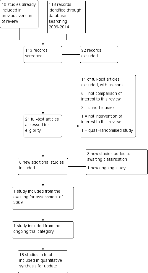
Study flow diagram for 2009 to 2013 literature searches.
The study characteristics and inclusion and exclusion criteria for each study are described in the tables Characteristics of included studies and Characteristics of excluded studies.
Included studies
Eighteen studies were included in total (AboulGheit 2010; Andrés‐Oros 2008; Claman 2004; da Silva 2012; Kyrou 2012; Lewis 2006; Lorusso 2008; Martinez 1991a; Martinez 1991b; Nikbakht 2012; Rahman 2011; Sakhel 2007; Scott 1994; Shalev 1995; Sharma 2011; Schmidt‐Sarosi 1995; Weiss 2010; Zreik 1999) (see Characteristics of included studies). Twelve compared different synchronisation approaches, four compared the optimum time interval from the onset of hCG injection to IUI (AboulGheit 2010; Claman 2004; Rahman 2011; Weiss 2010), one study compared different dosages of hCG injection (Nikbakht 2012) and one study compared early hCG injection (dominant follicle of 16.0 to 16.9 mm) with late hCG injection (dominant follicle 18.0 to 18.9 mm) (da Silva 2012). The study of Lewis 2006, both studies of Martinez 1991a, and the study of Zreik 1999 were used in a meta‐analysis to compare the methods of urinary LH surge versus hCG injection (264 women, 242 first cycle treatments). The study of Kyrou 2012 compared the methods of serum LH detection versus hCG injection in natural cycles. All other studies used some form of ovarian stimulation. Two studies (Lorusso 2008; Sakhel 2007) compared the use of recombinant hCG versus urinary hCG (409 women, 441 cycles) and five studies (Andrés‐Oros 2008; Schmidt‐Sarosi 1995; Scott 1994; Shalev 1995; Sharma 2011) compared the use of hCG versus a GnRH agonist for timing IUI (4 studies, 206 women, 486 cycles). The abstract of Sharma 2011 reported 450 included women but the number of cycles was unclear and the pregnancy rates were expressed in percentages only. Therefore the study was not included in the meta‐analysis. The study of Claman 2004 was not used in a meta‐analysis because only per cycle data were available (75 women, 189 cycles). The study of Kyrou 2012 was not used in the meta‐analysis since more than half of the women underwent insemination for other reasons than subfertility, and there were no data available for the group with subfertility alone (Kyrou 2012). Finally, the study of Weiss 2010 was not included in the meta‐analysis since data per cycle were available with couples who dropped out after randomisation excluded from the analysis (see Characteristics of included studies).
Participants
The age of the participants was stated in all but one trial (Sharma 2011) as either a mean with the standard deviation (SD) for each treatment group or overall. The mean age ranged from 26 to 34 years. There were no statistical differences recorded between the various treatment groups based on age.
All studies included different types of subfertility: unexplained subfertility, mild endometriosis, male factor, cervical factor and tubal or pelvic factor. The study population of Kyrou 2012 contained 58% of women without subfertility (lesbian, single mother) as stated above. Seven studies (Claman 2004; Nikbakht 2012; Sakhel 2007; Schmidt‐Sarosi 1995; Shalev 1995; Weiss 2010; Zreik 1999) also included women with ovulatory disorders. In the studies of Claman 2004 and Zreik 1999 the women with ovulatory disorders comprised less than 15% of all women. In the studies of Sakhel 2007 and Schmidt‐Sarosi 1995 these women comprised around 25% of the total group. In the study of Shalev 1995 69% of the total group of participants had cycle disorders. In all five studies they were equally distributed between the two treatment arms. In the studies of Nikbakht 2012 and Weiss 2010 the number and distribution of these women were not described. Finally, the study of da Silva 2012 included a category 'female factor' (23.4%) without describing details of this group.
The duration of subfertility was given in 10 trials (AboulGheit 2010; da Silva 2012; Lorusso 2008; Martinez 1991a; Martinez 1991b; Nikbakht 2012; Rahman 2011; Sakhel 2007; Weiss 2010; Zreik 1999). In two studies (AboulGheit 2010; Sakhel 2007) the duration was significantly different between the treatment groups. AboulGheit 2010 reported a mean duration of subfertility of 5.6 years in the 24 hours after hCG group compared to a mean of 3.1 and 3.5 years in the 34 hours and 48 hours after hCG groups. Although the pregnancy rates in the first group were lower compared to the other groups, this was not significant. Sakhel 2007 reported a longer duration of subfertility in the group treated with urinary hCG. This difference still remained a factor after analysing the data using logistic regression analysis with clinical pregnancy rate as the dependent variable and controlling for duration of infertility. They did not state if the difference was of any clinical relevance. In the studies of Martinez and co‐workers the mean duration of subfertility was 5.6 and 6.3 years, which was quite long and could have negatively influenced their outcome parameters.
Four studies (da Silva 2012; Nikbakht 2012; Sakhel 2007; Weiss 2010) mentioned the number of couples with primary versus secondary subfertility. Their populations contained between 36% and 68.5% with primary subfertility.
Eight studies (da Silva 2012; Kyrou 2012; Lewis 2006; Martinez 1991a; Schmidt‐Sarosi 1995; Shalev 1995; Sharma 2011; Zreik 1999) stated that they had included women who had undergone previous fertility treatment. Most of the women in the studies of Lewis 2006, Schmidt‐Sarosi 1995 and Zreik 1999 had been treated with clomiphene citrate without IUI. Three studies (da Silva 2012; Martinez 1991a; Sharma 2011) included women who previously had undergone IUI treatment cycles. Kyrou 2012 and Shalev 1995 did not mention the type of previous fertility treatment.
Interventions
Three (Lewis 2006; Martinez 1991b; Zreik 1999) of the four studies comparing urinary LH versus hCG injection used clomiphene citrate as a method of ovarian stimulation. Clomiphene citrate was used either from cycle days three to seven or cycle days five to nine. The fourth study used HMG (Martinez 1991a). One study compared serum LH versus hCG injection in a natural cycle (Kyrou 2012). The studies Lorusso 2008 and Sakhel 2007 comparing recombinant hCG (r‐hCG) with urinary hCG (u‐hCG) both used recombinant FSH (r‐FSH) for ovarian stimulation. However, Sakhel 2007 also added hMG and when the E2 level exceeded 300 pg/mL, or a leading follicle of more than 14 mm diameter was present, a gonadotropin‐releasing hormone antagonist was applied. The studies comparing hCG with a GnRH agonist (Andrés‐Oros 2008; Schmidt‐Sarosi 1995; Scott 1994; Shalev 1995; Sharma 2011) used different ovarian stimulation protocols including clomiphene citrate (Schmidt‐Sarosi 1995; Scott 1994; Sharma 2011), FSH (Andrés‐Oros 2008) and hMG (Shalev 1995). Different stimulation protocols were also used in the studies trying to define the optimal timing of IUI. Rahman 2011 used clomiphene citrate as a method of ovarian stimulation, Claman 2004 and Weiss 2010 used hMG or r‐FSH. Only AboulGheit 2010 compared the optimal timing of IUI after hCG in natural cycles. The study of da Silva 2012 compared early hCG with late hCG depending on the size of the dominant follicle, stimulated with highly purified HMG. Finally, the study of Nikbakht 2012 comparing two doses of r‐hCG achieved ovarian hyperstimulation with clomiphene citrate or letrozole and HMG
Urinary LH versus hCG injection
The use of the technique for timing IUI was one of the comparisons of interest in this review. Lewis 2006 included one group of women which used a home ovulation predictor kit once a day: in the afternoon, starting on day 12. Insemination was scheduled the morning after the first positive test. The women in the hCG group started ultrasound monitoring on day 12 and 10,000 IU hCG was given when there was at least one follicle with a mean diameter of 20 mm and the endometrial thickness was at least 8 mm. A single IUI was scheduled 33 to 42 hours later. Any woman who did not satisfy criteria for hCG administration was instructed to perform home monitoring for an LH surge until their next ultrasound, and to schedule an insemination if her predictor kit gave a positive result. There were no details on how often LH surges were detected in the ultrasound group before a follicle reached the size of 20 mm.
Martinez 1991a started daily ultrasound scanning when total urinary estradiol excretion exceeded 200 mmol/24 hours. When the largest follicle reached a diameter between 18 and 20 mm on ultrasound and the total estradiol excretion was between 300 and 1200 nmol/24 hours women received 10,000 IU hCG. LH detection in the urine was done twice daily from the moment the dominant follicle reached the size of 15 mm. A single IUI was performed 36 to 40 hours after hCG administration or 16 to 28 hours after urinary LH surge detection.
Martinez 1991b started urinary LH monitoring twice a day when the dominant follicle had reached 15 mm in diameter. Women were inseminated 21 hours after an evening positive urine or 24 hours after a morning positive urine. The other treatment group received 10,000 IU hCG when the dominant follicle reached a diameter size between 18 and 22 mm, measured daily by ultrasound when a dominant follicle had reached the size of 15 mm. From 37 to 40 hours after hCG a single IUI was performed.
Zreik 1999 started urinary LH monitoring in the morning on day 10 of the cycle. Ultrasound monitoring in the hCG group started on day 10 and 10,000 IU hCG was given when a leading follicle with diameter 18 mm diameter was noted. In both groups IUI was performed daily for the next two days.
Serum LH versus hCG injection
Kyrou 2012 was the only study using serum LH testing instead of urinary LH testing. The daily monitoring of serum LH levels could start from day 6 of the cycle until the LH rise. When LH started to rise, a second assessment was performed the next day to confirm the LH rise. Criteria for detection were an LH rise of 180% above the latest serum value. In the hCG group women received 5000 IU of hCG as soon as a follicle reached a diameter of ≥ 17 mm. A single IUI was performed 36 h after initiation of the LH rise or 36 h after the hCG injection. In the case where the serum LH suggested an imminent ovulation (LH rise and rise in progesterone) the insemination was performed after 24 h.
Recombinant hCG (r‐hCG) versus urinary hCG (u‐hCG)
Lorusso 2008 monitored ovarian response by ultrasound only. Urinary or recombinant hCG was given when one follicle with a mean diameter of 18 mm or more was present or no more than three follicles had a mean diameter of 16 mm. Double IUI was carried out 24 and 48 hours after administration, except when ovulation had occurred after 24 hours.
Sakhel 2007 monitored ovarian response by ultrasound and serum PGE2. When two or more follicles were 16 mm, with 200 pg/mL E2 per follicle, 10,000 IU u‐hCG or 250 mg r‐hCG was used to induce ovulation. A single IUI was performed 42 hours after the injection but this could be delayed by four hours when there was no collapse of the leading follicle observed on ultrasound. Luteal support was added with progesterone.
hCG versus GnRH agonist (GnRH‐a)
Andrés‐Oros 2008 administered a single injection of triptorelin (0.2 mg) or a single injection of r‐hCG (250 µg) when at least one follicle, and not more than three, reached the size 18 mm or more. A single IUI was performed 36 hours after the injection. Luteal support with progesterone was applied.
Schmidt‐Sarosi 1995 began ultrasound monitoring from cycle day 11. When the largest follicle was > 20 mm, 400 µg nafarelin intranasally (IN) was given on this and the following day, IUI was performed 48h after the first dose. The hCG group received an intramuscular injection of 5000 IU when the largest follicle reached > 20 mm and IUI was performed after 36 h. Luteal support in the GnRH‐a group was given as seven doses of 400 µg nafarelin every 16 hours started 6 days after the first dose. Women in the hCG group received one injection of 2500 IU hCG six days after the primary injection.
Scott 1994 started daily pelvic ultrasound on cycle day 12. When the dominant follicle reached a diameter of 20 to 21 mm the women received GnRH‐a (2 mg leuprolide acetate) subcutaneously or 10,000 IU hCG intramuscularly. Approximately 40 hours after injection, these women underwent a single IUI after a pelvic ultrasound was performed.
Shalev 1995 administered a single injection of triptorelin (0.1 mg) or single injection hCG (10,000 IU) when at least one follicle attained a diameter of 16 mm. Double IUI was performed 24 and 48 hours after the injection.
Sharma 2011 started follicle monitoring from cycle day 10. Urinary hCG (5000 IU) or GnRH‐a (leuprolide 1 mg) was given when a follicular diameter was between 18 and 20 mm with endometrial thickness ≥ 7 mm. A single IUI was performed only after confirmation of ovulation with ultrasound. Luteal support was given with 300 mg vaginal micronized progesterone daily for 15 days.
Optimal time interval
Four studies compared the optimum time interval from ovulation induction to IUI. AboulGheit 2010 triggered ovulation with highly purified hCG (Choriomon, 10,000 IU) intramuscular injection when the leading follicle reached ≥ 18 mm and when at least two follicles reached ≥ 16 mm. Timing of IUI was 24 hours, 34 hours and 48 hours after hCG.
In the study of Claman 2004 the women received 5000 IU hCG intramuscularly or 10,000 IU hCG subcutaneously when two to five follicles were seen on ultrasound with a mean diameter of 17 to 21 mm. Timing of IUI was between 32 and 34 hours or 38 and 40 hours after hCG.
Rahman 2011 started ultrasound monitoring from cycle day 11 or earlier depending on the women’s cycles. An ovulation trigger was given with injection of 5000 IU hCG when at least one follicle reached 18 mm or more and endometrial thickness was at least 7 mm. Single insemination was performed 24 or 36 hours after hCG injection.
Weiss 2010 administered hCG after a cycle with mild ovarian stimulation using gonadotropins and GnRH antagonist. The time and amount of hCG administered was not mentioned, but if five or more follicles over 15 mm were developed, or if ovulation took place before administration of the GnRH antagonist, the couple was excluded. Insemination took place 36 h, 42 h or 48 h after hCG administration. Luteal support was given with endometrin 100 mg twice a day from insemination until eight weeks of gestation.
Size of follicle at hCG injection
da Silva 2012 administered HMG from cycle day 4. Dose adjustments were made according to ovarian response until the criteria for hCG administration were met; 5000 IU of hCG was injected when the dominant follicle was between 16.0 and 16.9 mm diameter and 18.0 and 18.9 mm, respectively, and approximately 36 hours later IUI was performed. Luteal support was obtained with natural micronized progesterone 600 mg/day vaginally.
Two doses of recombinant hCG
In Nikbakht 2012 clomiphene or letrozole and HMG (Pergonal) were administered. When two or more follicles were 16 mm, r‐hCG 250 or 500 ug was used to induce ovulation. A single IUI was performed 42 hours after r‐hCG injection.
The studies used partners' semen, although this was not noted explicitly in all studies. Three studies noted donor cycles (Kyrou 2012; Lewis 2006; Weiss 2010). Semen preparation techniques, the amount of semen fluid injected, the number of motile semen injected and the type of insemination catheter were poorly described or not described at all (see table Characteristics of included studies).
Outcomes
Seven trials (Martinez 1991a; Rahman 2011; Sakhel 2007; Schmidt‐Sarosi 1995; Scott 1994; Shalev 1995; Weiss 2010) reported live birth rates. All but one trial (Claman 2004) assessed pregnancy rate per couple. In one study (Weiss 2010) the couples who dropped out after inclusion were not included in the calculation of the live birth rate and pregnancy rate per couple. Therefore, the latter study was excluded from the meta‐analysis.
Multiple pregnancy rates and miscarriage rates were reported in 11 studies (Andrés‐Oros 2008; da Silva 2012; Lewis 2006; Lorusso 2008; Martinez 1991a; Martinez 1991b; Sakhel 2007; Schmidt‐Sarosi 1995; Scott 1994; Shalev 1995; Weiss 2010). AboulGheit 2010 reported chemical pregnancies and clinical pregnancies separately. The OHSS rate was stated in five studies (Lorusso 2008; Martinez 1991a; Sakhel 2007; Schmidt‐Sarosi 1995; Shalev 1995) and the ectopic pregnancy rate was stated in two publications (Sakhel 2007; Weiss 2010).
One of the studies assessed the costs of the treatment (Lewis 2006). The cost per pregnancy in the LH group was estimated to be USD 3695 and the cost per pregnancy in the hCG group was USD 4830.
Four studies (AboulGheit 2010; Lewis 2006; Nikbakht 2012; Sakhel 2007) diagnosed pregnancy by a rising concentration of hCG. In two studies (Lewis 2006; Rahman 2011) the pregnancy was called viable when a fetal pole with cardiac activity was noted on ultrasound. Five studies (AboulGheit 2010; da Silva 2012; Martinez 1991a; Martinez 1991b; Nikbakht 2012) stated that an ultrasound detection of fetal heart rate activity was performed four weeks after conception and in the study of Kyrou and co‐workers ultrasound detection of fetal heart rate activity was performed 10 weeks after conception. Five studies (Andrés‐Oros 2008; Lorusso 2008; Shalev 1995; Sharma 2011; Weiss 2010) defined clinical pregnancy by the presence of a gestational sac in the uterus, determined by transvaginal ultrasound. Three studies (Schmidt‐Sarosi 1995; Scott 1994; Zreik 1999) did not mention the method of confirming pregnancy.
Studies awaiting assessment
All studies previously awaiting assessment were included (noting that the risk of bias was high, see table Characteristics of included studies).
Attempts have been made to contact authors to get further information about the methods of randomisation, to retrieve unpublished data and for details about published data. Eight replies have been received, resulting in exclusion of four trials (Diaz 2003a; Diaz 2003b; Lewis 2003; Pierson 2002) and inclusion of three trials (Scott 1994; Shalev 1995; Weiss 2010).
Four new studies (Aydin 2013; Blockeel 2014; Dehghani 2014; Mostafa 2014) that were identified will be assessed when this review is next updated.
Ongoing trials
One trial with the comparison of interest is registered on the ClinicalTrials.gov database and is still recruiting couples (OVO R&D 2012) (see Characteristics of ongoing studies). One of the ongoing trials of the 2009 review has been included (Weiss 2010).
Excluded studies
Fifty‐five studies were excluded (see table Characteristics of excluded studies). Reasons for exclusion were: failure to use a truly randomised design (n = 19) (Agarwal 1995; Cedrin‐Durnerin 1993; Check 1994; Costa Franco 2006; Diaz 2003a; Diaz 2008; Fondop 2005; Gerris 1995; Ghanem 2011; Khattab 2005; Kossoy 1989; Martinez 1994; Meherji 2004; Panchal 2009; Romeu 1997a; Romeu 1997b; Shanis 1995; Tavaniotou 2003; Tonguc 2010), not performing the comparison of interest (n = 18) (Arici 1994; Baroni 2001; Casadei 2006; Federman 1990; Fischer 1993; Gerrits 2011; Ghazizadeh 2009; Ghosh Dastidar 2009; Kotecki 2005; Nulsen 1993; Papageorgiou 1995; Pierson 2002; Pirard 2005; Ragni 1999; Ramon 2009; Robinson 1992; Silverberg 1991; Wang 2006), not performing IUI (n = 5) (Barratt 1989; Claraz 1989; George 2007; Odem 1991; Scarpellini 1991), did not meet the inclusion criteria for types of participants (n = 2) (Egbase 2003; Int rhCG study group 2001), or duplicate publications of abstracts or full text articles (n = 8) (Claman 2000; Claman 2004a; Diaz 2003b; Lewis 2002; Lewis 2003; Ramon 2009a; Sakhel 2004; Wang 2001). Finally, one study was excluded from the awaiting assessment category since we did not receive the information we needed about the randomisation method (n = 1) (Propst 2007). The same authors published an abstract in 2012 on the same subject. The research population described seems to be the same group as published before. Additional information was lacking, thus this abstract was excluded as well (Propst 2012).
Risk of bias in included studies
Figure 2 presents our judgements about each methodological quality item, presented as percentages across all included studies, and Figure 3 summarises our judgements about each methodological quality item for each included study.
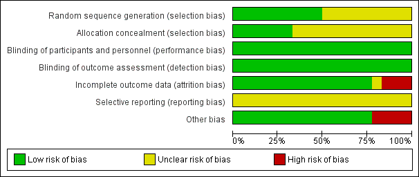
Methodological quality graph: review authors' judgements about each methodological quality item presented as percentages across all included studies.
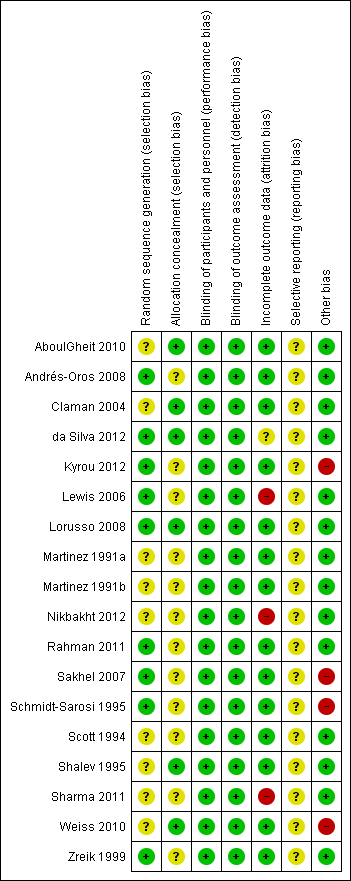
Methodological quality summary: review authors' judgements about each methodological quality item for each included study.
Study design
Four studies (Martinez 1991a; Martinez 1991b; Scott 1994; Zreik 1999) used a cross‐over design, with pre‐cross over data available. For the meta‐analysis we only included the first cycle data from these cross‐over studies. The trial design was parallel group in the other included studies.
Allocation
The description of methods for randomisation or allocation concealment was generally poor in the published information, which might increase the risk for selection bias. However, additional information was received about allocation methods for most studies.
Random sequence generation
Nine studies mentioned the use of a computer generated program for randomisation (Andrés‐Oros 2008; da Silva 2012; Kyrou 2012; Lewis 2006; Lorusso 2008; Rahman 2011; Sakhel 2007; Shalev 1995; Weiss 2010; Zreik 1999). Five studies (Claman 2004; Martinez 1991a; Martinez 1991b; Schmidt‐Sarosi 1995; Scott 1994) used a random number table, not further specified. Two studies (Nikbakht 2012; Sharma 2011) reported a random assignment without further specification.
Allocation concealment
Concealment of allocation was stated explicitly in six studies (AboulGheit 2010; da Silva 2012; Lewis 2006; Lorusso 2008; Weiss 2010; Zreik 1999). After additional information about allocation had been received, seven other trials (Andrés‐Oros 2008; Claman 2004; Martinez 1991a; Martinez 1991b; Sakhel 2007; Scott 1994; Shalev 1995) could be deemed at low risk of bias in this domain. Concealment of allocation was done by the use of sealed opaque envelopes or a third party (Figure 2; Figure 3). Two studies (Nikbakht 2012; Sharma 2011) were deemed at high risk of this bias. Concealment of allocation was done with sealed envelopes in the latter study.
Blinding
In two studies (Scott 1994; Shalev 1995) blinding was performed. Scott and co‐workers used blinding of the sonographer to minimise the risk of observer bias in determining if ovulation had taken place after injection of hCG or GnRH‐a. None of the trials had details on blinded analysis of the results. All studies were rated at low risk of bias with respect to blinding as we determined that it was unlikely to influence our review outcomes.
Incomplete outcome data
Nine studies reported information on dropouts (Claman 2004; da Silva 2012; Kyrou 2012; Lewis 2006; Martinez 1991a; Martinez 1991b; Weiss 2010; Zreik 1999). The number of dropouts varied from 0% to 31%. Additional information on dropouts was received from four studies (Andrés‐Oros 2008; Sakhel 2007; Shalev 1995; Weiss 2010). The first study (Andrés‐Oros 2008) reported the dropping out of 18 couples who did not meet the criteria to induce ovulation (too many follicles, or no follicles). The main reason for dropout in the study of Weiss and co‐workers was a transfer to in vitro fertilisation (IVF) because of overstimulation. The other five studies reported no dropouts.
Claman and co‐workers stated that the most important reasons for dropping out were a spontaneous LH surge or an inadequate follicular response. Lewis and co‐workers noted failure to detect an LH surge in 23% of the participants in the LH group. In the hCG group 5.3% of the participants dropped out due to personal reasons, especially because of time commitment. An ITT analysis was performed resulting in no significant difference between the treatment groups. In the study of Zreik and co‐workers only one couple out of 54 was excluded, due to failure in compliance. None of the included women in the studies by Martinez 1991b and Kyrou 2012 dropped out. The other study of Martinez (Martinez 1991a) reported that five women decided to stop after the second cycle, and five did not complete the third cycle. Finally, the study of da Silva 2012 reported major protocol deviations in 117/635 couples, no hCG due to insufficient follicular growth in 61/635 couples, and serum estradiol (E2) > 1500 pg/ml or premature LH peak (LH > 10 mIU/ml). No explanation for protocol deviation was reported.
Selective reporting
A total of 44% of the included studies reported live birth rates. The remaining studies defined clinical pregnancy rates (see table Characteristics of included studies).
Other potential sources of bias
Sakhel and co‐workers reported that the included women in the u‐hCG group had a greater mean duration of infertility than the r‐hCG group, which may have been a source of bias in this study. The same applies to the study of AboulGheit 2010 where the couples in the IUI 24 hours after hCG group had a longer mean duration of infertility. Weiss and co‐workers reported significantly more miscarriages in the group with a time interval of 36 hours, and the study of Kyrou and co‐workers included a high percentage of non‐subfertile women. da Silva 2012 did not report the exact size of the dominant follicles per group, which might have introduced bias. Finally, Sharma 2011 excluded 20 couples before randomisation for unclear reasons.
Effects of interventions
See: Summary of findings for the main comparison hCG compared to LH surge for intrauterine insemination in subfertile couples; Summary of findings 2 u‐hCG compared to r‐hCG for intrauterine insemination in subfertile couples; Summary of findings 3 Short interval compared to long interval for intrauterine insemination in subfertile couples; Summary of findings 4 hCG compared to GnRH‐a for intrauterine insemination in subfertile couples; Summary of findings 5 Early hCG compared to late hCG for intrauterine insemination in subfertile couples; Summary of findings 6 Differing dosages of hCG for intrauterine insemination in subfertile couples
Overall 18 studies with a total of 2279 couples were included in the review.
1. hCG versus LH surge
Four studies compared hCG with LH surge for timing IUI (Lewis 2006; Martinez 1991a; Martinez 1991b; Zreik 1999).
1.1 Live birth rate
One study (Martinez 1991a) reported live birth rate. There was no evidence of a difference between hCG and LH surge (odds ratio (OR) 1.0, 95% confidence interval (CI) 0.06 to 18.08; 1 trial, 24 women, very low quality evidence) (Analysis 1.1).
1.2 Pregnancy rate
All trials included for this comparison reported pregnancy rate per couple. The result revealed no evidence of a difference in pregnancy rate per couple (OR 1.33, 95% CI 0.72 to 2.45; 4 trials, 275 women, I2 = 0%, low quality evidence) (Analysis 1.2, Figure 4).
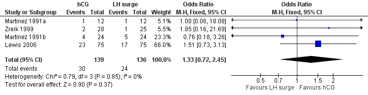
Forest plot of comparison: 1 hCG versus LH surge, outcome: 1.2 pregnancy rate per couple.
1.3 Multiple pregnancy rate
The meta‐analysis of two studies (Lewis 2006; Martinez 1991a) revealed no evidence of a difference in multiple pregnancy rates (OR 1.12, 95% CI 0.17 to 7.6; 2 trials, 42 pregnancies, very low quality evidence) (Analysis 1.3).
2. u‐hCG versus r‐hCG
Two studies (Lorusso 2008; Sakhel 2007) compared u‐hCG with r‐hCG for timing IUI.
2.1 Live birth rate
One study (Sakhel 2007) reported live birth rate, which showed no evidence of a difference between u‐hCG and r‐hCG (OR 1.17, 95% CI 0.68 to 2.03; 1 trial, 284 women, low quality evidence) (Analysis 2.1).
2.2 Pregnancy rate
All trials included in this comparison reported pregnancy rate per couple. The result revealed no evidence of a difference in pregnancy rate per couple (OR 1.02, 95% CI 0.65 to 1.57; 2 trials, 409 women, I2 = 0%, low quality evidence) (Analysis 2.2, Figure 5).
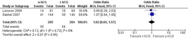
Forest plot of comparison: 2 u‐hCG versus r‐hCG, outcome: 2.2 pregnancy rate per couple.
2.3 Multiple pregnancy rate
No evidence of a difference in multiple pregnancy rates was reported (OR 0.99, 95% CI 0.4 to 2.47; 2 trials, 109 pregnancies, low quality evidence) (Analysis 2.3).
2.4 Miscarriage rate
Miscarriages per treatment group showed no evidence of a difference between groups (OR 0.57, 95% CI 0.13 to 2.47; 2 trials, 109 pregnancies, I2 = 0%, very low quality evidence) (Analysis 2.4, Figure 6).

Forest plot of comparison: 2 u‐hCG versus r‐hCG, outcome: 2.4 miscarriage rate per pregnancy.
2.5 OHSS rate
Both studies reported no cases of (severe) OHSS in a total of 468 cycles (moderate quality evidence) (Analysis 2.5).
3. Short versus long interval
Two studies (AboulGheit 2010; Rahman 2011) compared a short interval (24 hours) with a long interval (34 to 36 hours) after hCG. AboulGheit 2010 included a third group (IUI 48 hours after hCG).
3.1 Live birth rate
One study (Rahman 2011) reported live birth rate, which showed no evidence of a difference between IUI after 24 hours and 34 hours (OR 0.52, 95% CI 0.27 to 1.00; 1 trial, 204 couples, low quality evidence) (Analysis 3.1).
3.2 Pregnancy rate
Both studies reported pregnancy rate per couple. The meta‐analysis revealed a lower pregnancy rate in the 24 hour group, when IUI was after 24 hours compared with IUI after 34 to 36 hours (OR 0.55, 95% CI 0.31 to 0.98; 2 trials, 234 women, I2 = 0%, low quality evidence) (Analysis 3.2). AboulGheit 2010 also compared IUI after 24 hours with IUI after 48 hours and found no evidence of a difference between the groups (OR 0.44, 95% CI 0.10 to 1.92; 1 trial, 30 women, low quality evidence) (Analysis 3.2). Nor was there a diffference between IUI after 34 to 36 hours and IUI after 48 hours (OR 0.58, 95% CI 0.14 to 2.48; 1 trial, 30 women, low quality evidence) (Analysis 3.2, Figure 7).
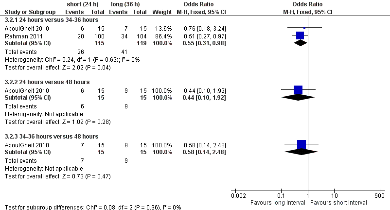
Forest plot of comparison: 3 short versus long interval, outcome: 3.2 pregnancy rate per couple.
3.3 Miscarriage rate
Both studies reported miscarriage rates, with no evidence of a difference between the groups of 24 hours versus 34 to 36 hours (OR 1.58, 95% CI 0.35 to 7.16; 2 trials, 67 pregnancies, I2 = 0%, very low quality evidence); 24 hours versus 48 hours (OR 4.0, 95% CI 0.27 to 58.56; 1 trial, 15 women, very low quality evidence); 34 to 36 hours versus 48 hours (OR 1.33, 95% CI 0.07 to 25.91; 1 trial, 16 women, very low quality evidence) (Analysis 3.3) respectively. Two studies (Claman 2004; Weiss 2010) were excluded from the meta‐analysis since they reported results as pregnancy rates per cycle only. The former did not report a difference between 32 to 34 hours and 38 to 40 hours after hCG, and the latter study was stopped prematurely because of an unusual number of multi‐fetal pregnancies; the study reported a higher pregnancy rate for 42 hours after hCG compared to 36 hours or 48 hours (see table 'Characteristics of included studies' for details, Figure 8).
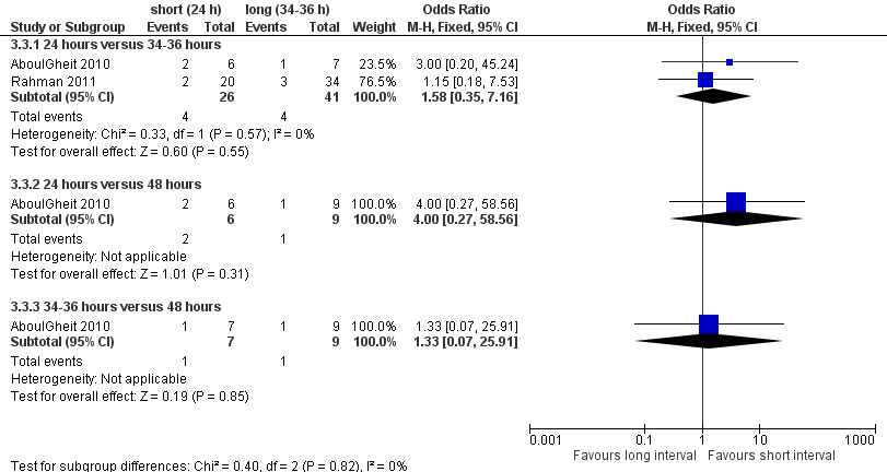
Forest plot of comparison: 3 short versus long interval, outcome: 3.3 miscarriage rate per pregnancy.
4. hCG versus GnRH‐a
Four studies (Andrés‐Oros 2008; Schmidt‐Sarosi 1995; Scott 1994; Shalev 1995) compared hCG versus GnRH‐a.
4.1 Live birth rate
The results for live birth rate per couple revealed no evidence of a difference between the groups (OR 1.04, 95% CI 0.42 to 2.56; 3 trials, 104 women, I2 = 0%, low quality evidence) (Analysis 4.1, Figure 9).
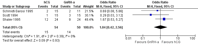
Forest plot of comparison: 4 hCG versus GnRH‐a, outcome: 4.1 live birth rate per couple.
4.2 Pregnancy rate
All trials reported the pregnancy rate per couple revealing no evidence of a difference between groups (OR 1.14, 95% CI 0.63 to 2.08; 4 trials, 206 women, I2 = 48%, low quality evidence) (Analysis 4.2, Figure 10).
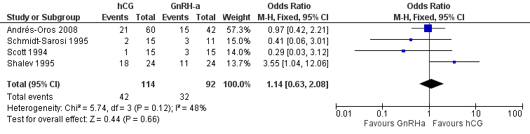
Forest plot of comparison: 4 hCG versus GnRH‐a, outcome: 4.2 pregnancy rate per couple.
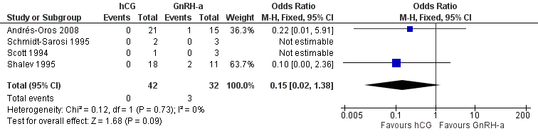
4.3 Multiple pregnancy rate
The studies reported three twin pregnancies in the GnRH‐a group and none in the hCG group. There was no evidence of a difference in multiple pregnancy rates between hCG and GnRH‐a (OR 0.15, 95% CI 0.02 to 1.38; 4 trials, 74 pregnancies, I2 = 0%, very low quality evidence) (Analysis 4.3, Figure 11).
Forest plot of comparison: 4 hCG versus GnRH‐a, outcome: 4.3 multiple pregnancy rate per pregnancy.
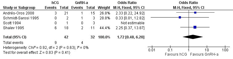
4.4 Miscarriage rate
There was no evidence of a difference in the miscarriage rate between the GnRH‐a and hCG group (OR 1.72, 95% CI 0.48 to 6.2; 4 trials, 74 pregnancies, I2 = 0%, very low quality evidence) (Analysis 4.4, Figure 12).
Forest plot of comparison: 4 hCG versus GnRH‐a, outcome: 4.4 miscarriage rate per pregnancy.
4.5 OHSS rate
OHSS rates were compared and there was no evidence of a difference between groups (OR 2.27, 95% CI 0.65 to 7.91; 3 trials, 456 women, low quality evidence) (Analysis 4.5). Shalev 1995 reported four treatment cycles with grade three to grade four OHSS in the GnRH‐a group, and eight treatment cycles with OHSS in the hCG group; the other two studies in this meta‐analysis reported none in either group.
5. Early versus late hCG
One study (da Silva 2012) compared early hCG versus late hCG.
5.1 Pregnancy rate
No evidence of a difference was reported between both treatment groups in the pregnancy rate per couple (OR 1.32, 95% CI 0.77 to 2.25; 1 trial, 612 women, low quality evidence) (Analysis 5.1).
5.2 Miscarriage rate
No evidence of a difference between miscarriages rates was reported (OR 0.51, 95% CI 0.08 to 3.28; 1 trial, 65 pregnancies, very low quality evidence) (Analysis 5.2).
The authors reported two multiple pregnancies in the early hCG group and none in the late hCG group.
6. Different dosages of hCG
One trial (Nikbakht 2012) compared 250 ug r‐hCG with 500 ug r‐hCG.
6.1 Pregnancy rate
No evidence of a difference in pregnancy rate per couple was reported (OR 1.38, 95% CI 0.28 to 6.71; 1 trial, 66 women, very low quality evidence) (Analysis 6.1).
Discussion
Summary of main results
The aim of this review was to investigate the optimal synchronisation of ovulation with intrauterine insemination (IUI) in subfertile couples undergoing natural and stimulated cycles with regard to live birth rates. The trials in this review revealed that not one of the available methods is superior to another. However, the available evidence is scarce due to small sample sizes and lack of data concerning the primary outcome.
hCG injection versus LH surge detection
Although the dropout rate in the LH surge group was much higher than in the hCG group (due to no detection of a LH surge in 23% of the cycles) there was no evidence of a difference in live birth or pregnancy rates between these treatment groups (OR 1.5, 95% CI 0.73 to 3.1) (Lewis 2006).
The cause of dropouts in the LH surge group could be the absence of detection of LH surges in urine samples. This has been reported in other studies as well, due to a short LH surge or incorrect use of the intervention by the woman (Miller 1996). When counselling couples, the advantages of home ovulation predictor tests (no difference in pregnancy outcomes compared to hCG injection, convenience and low costs) and disadvantages (high number of false‐negative results) should be considered in relationship to the advantages (low number of false‐negative results) and disadvantages (expensive and time consuming) of ultrasound detection combined with hCG injection. No data on the occurrences of premature LH surges in the hCG group have been reported in the pooled studies. This might negatively influence the treatment outcome in the hCG group, resulting in lower pregnancy rates and no perceptible difference between timing using LH surge detection and hCG injection (Cantineau 2007).
The general quality of the evidence was estimated to be low or very low, meaning that further research is likely or very likely to have an important impact on our confidence in the estimate of effect and is likely to change this estimate (summary of findings Table for the main comparison).
Urinary hCG (u‐hCG) versus recombinant hCG (r‐hCG)
No evidence of a difference in pregnancy rates was found between u‐hCG and r‐hCG. Other reasons such as costs, injection site reactions and possible batch‐to‐batch inconsistencies should be considered in deciding which to use.
The general quality of the evidence was estimated to be low or very low (summary of findings Table 2).
Short (24 hours) versus long interval (36 hours)
The evidence provided by prospective studies (AboulGheit 2010; Rahman 2011) comparing different hCG to IUI intervals after ovarian stimulation revealed more live births when an interval of 34 to 36 hours was used. However, this difference was not statistically significant. A higher number of pregnancies was reported when IUI was performed 34 to 36 hours after hCG compared to IUI 24 hours after hCG injection. This might be in part due to a significant difference in the duration of subfertility (significantly longer in the 24 hours group in the study of AboulGheit 2010). This study and other studies that only reported pregnancy rate per cycle suggest a more flexible approach in timing IUI after hCG, which allows women to inject hCG in the early evening when pharmacies are still open, in case of problems (Claman 2004).
The general quality of the evidence was estimated to be low or very low (summary of findings Table 3).
hCG versus GnRH agonist (GnRH‐a)
No evidence of a difference was found, when analysing live birth rates and pregnancy rates, between the timing methods using hCG and GnRH‐a. More evidence is needed to determine the place of GnRH‐a as a timing method for IUI, also considering costs and secondary outcomes such as the OHSS rate.
The general quality of the evidence was estimated to be low or very low (summary of findings Table 4).
Early hCG versus late hCG depending on the size of the dominant follicle
As well as the ITT analysis, the per protocol analysis reported no advantage of hCG injection with a dominant follicle between 16.0 and 16.9 mm compared to a dominant follicle between 18.0 and 18.9 mm (da Silva 2012). Significantly more dominant follicles and significantly higher estradiol levels were seen in the late group without significantly increased numbers of premature LH surges or clinical pregnancies. No information was reported on the exact sizes of the dominant follicles. For example, when a dominant follicle was 17 mm in the early group it was unclear whether it was stated as a major protocol deviation. Since the day of hCG administration and the total dose of HMG did not differ, it is questionable how different the groups really were.
The general quality of the evidence was estimated to be low or very low (summary of findings Table 5).
Different dosages of hCG
No evidence of a difference was found between 250 µg r‐hCG and 500 µg r‐hCG. Significantly more dominant follicles were seen in the 250 µg r‐hCG group, which might be a confounding factor.
The quality of the evidence overall was estimated to be low or very low (summary of findings Table 6).
Overall completeness and applicability of evidence
Definite answers could not be given for most comparisons. When performing IUI, small numbers show a positive effect of insemination around 34 to 36 hours compared to 24 hours after hCG injection.
Quality of the evidence
The quality of the evidence for most comparisons was low or very low. The main limitations in the evidence were failure to describe study methods, serious imprecision and attrition bias.
Potential biases in the review process
Our searches aimed to identify all potentially eligible studies.
Agreements and disagreements with other studies or reviews
No other reviews were available concerning the difference between hCG injection and the LH detection test for timing IUI. Other retrospective studies revealed conflicting results.

Study flow diagram for 2009 to 2013 literature searches.

Methodological quality graph: review authors' judgements about each methodological quality item presented as percentages across all included studies.

Methodological quality summary: review authors' judgements about each methodological quality item for each included study.

Forest plot of comparison: 1 hCG versus LH surge, outcome: 1.2 pregnancy rate per couple.

Forest plot of comparison: 2 u‐hCG versus r‐hCG, outcome: 2.2 pregnancy rate per couple.
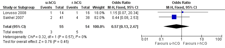
Forest plot of comparison: 2 u‐hCG versus r‐hCG, outcome: 2.4 miscarriage rate per pregnancy.

Forest plot of comparison: 3 short versus long interval, outcome: 3.2 pregnancy rate per couple.

Forest plot of comparison: 3 short versus long interval, outcome: 3.3 miscarriage rate per pregnancy.

Forest plot of comparison: 4 hCG versus GnRH‐a, outcome: 4.1 live birth rate per couple.

Forest plot of comparison: 4 hCG versus GnRH‐a, outcome: 4.2 pregnancy rate per couple.

Forest plot of comparison: 4 hCG versus GnRH‐a, outcome: 4.3 multiple pregnancy rate per pregnancy.

Forest plot of comparison: 4 hCG versus GnRH‐a, outcome: 4.4 miscarriage rate per pregnancy.

Comparison 1 hCG versus LH surge, Outcome 1 live birth rate per couple.

Comparison 1 hCG versus LH surge, Outcome 2 pregnancy rate per couple.

Comparison 1 hCG versus LH surge, Outcome 3 multiple pregnancy rate per pregnancy.

Comparison 2 u‐hCG versus r‐hCG, Outcome 1 live birth rate per couple.

Comparison 2 u‐hCG versus r‐hCG, Outcome 2 pregnancy rate per couple.

Comparison 2 u‐hCG versus r‐hCG, Outcome 3 multiple pregnancy rate per pregnancy.

Comparison 2 u‐hCG versus r‐hCG, Outcome 4 miscarriage rate per pregnancy.

Comparison 2 u‐hCG versus r‐hCG, Outcome 5 OHSS rate per cycle.
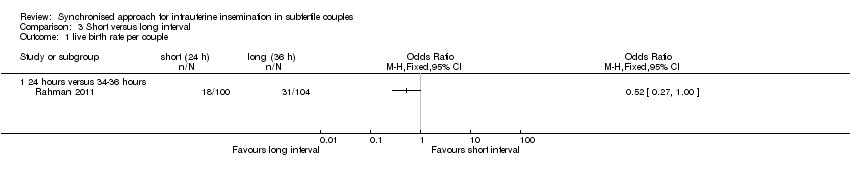
Comparison 3 Short versus long interval, Outcome 1 live birth rate per couple.

Comparison 3 Short versus long interval, Outcome 2 pregnancy rate per couple.

Comparison 3 Short versus long interval, Outcome 3 miscarriage rate per pregnancy.

Comparison 4 hCG versus GnRH‐a, Outcome 1 live birth rate per couple.

Comparison 4 hCG versus GnRH‐a, Outcome 2 pregnancy rate per couple.

Comparison 4 hCG versus GnRH‐a, Outcome 3 multiple pregnancy rate per pregnancy.

Comparison 4 hCG versus GnRH‐a, Outcome 4 miscarriage rate per pregnancy.

Comparison 4 hCG versus GnRH‐a, Outcome 5 OHSS per cycle.

Comparison 5 Early hCG versus late hCG, Outcome 1 pregnancy rate per couple.

Comparison 5 Early hCG versus late hCG, Outcome 2 miscarriage rate.

Comparison 6 Different dosages of hCG, Outcome 1 pregnancy rate per couple.
| hCG compared to LH surge for intrauterine insemination in subfertile couples | ||||||
| Population: women undergoing intrauterine insemination | ||||||
| Outcomes | Illustrative comparative risks* (95% CI) | Relative effect | No of participants | Quality of the evidence | Comments | |
| Assumed risk | Corresponding risk | |||||
| LH surge | HCG | |||||
| Live birth rate per couple | 83 per 1000 | 83 per 1000 | OR 1 | 24 | ⊕⊝⊝⊝ | |
| Pregnancy rate per couple | 146 per 1000 | 185 per 1000 | OR 1.33 | 275 | ⊕⊕⊝⊝ | |
| Multiple pregnancy rate per pregnancy | 59 per 1000 | 66 per 1000 | OR 1.12 | 42 | ⊕⊝⊝⊝ | |
| *The basis for the assumed risk was the median control group risk across studies. The corresponding risk (and its 95% confidence interval) is based on the assumed risk in the comparison group and the relative effect of the intervention (and its 95% CI). | ||||||
| GRADE Working Group grades of evidence | ||||||
| 1Methods used for random sequence generation and/or allocation concealment were unclear. 2There was very serious imprecision, with small sample sizes and very few events. 3There was serious imprecision: findings were compatible with substantial benefit in either group, or with no effect. | ||||||
| u‐hCG compared to r‐hCG for intrauterine insemination in subfertile couples | ||||||
| Population: women undergoing intrauterine insemination | ||||||
| Outcomes | Illustrative comparative risks* (95% CI) | Relative effect | No of participants | Quality of the evidence | Comments | |
| Assumed risk | Corresponding risk | |||||
| R‐hCG | U‐hCG | |||||
| Live birth rate per couple | 221 per 1000 | 249 per 1000 | OR 1.17 | 284 | ⊕⊕⊝⊝ | |
| Pregnancy rate per couple | 261 per 1000 | 265 per 1000 | OR 1.02 | 409 | ⊕⊕⊝⊝ | |
| Multiple pregnancy rate per pregnancy | 184 per 1000 | 182 per 1000 | OR 0.99 | 109 | ⊕⊕⊝⊝ | |
| Miscarriage rate per pregnancy | 84 per 1000 | 50 per 1000 | OR 0.57 | 109 | ⊕⊝⊝⊝ | |
| OHSS rate per cycle | See comment | See comment | Not estimable | 468 | ⊕⊕⊕⊝ | There were no events in either study |
| *The basis for the assumed risk was the median control group risk across studies. The corresponding risk (and its 95% confidence interval) is based on the assumed risk in the comparison group and the relative effect of the intervention (and its 95% CI). | ||||||
| GRADE Working Group grades of evidence | ||||||
| 1Methods used for random sequence generation and/or allocation concealment were unclear. 2There was serious imprecision: findings were compatible with substantial benefit in either group, or with no effect. 3One study did not report the method of allocation concealment used. 4There was very serious imprecision, with very few events and wide confidence intervals. | ||||||
| Short interval compared to long interval for intrauterine insemination in subfertile couples | ||||||
| Population: women undergoing intrauterine insemination | ||||||
| Outcomes | Illustrative comparative risks* (95% CI) | Relative effect | No of participants | Quality of the evidence | Comments | |
| Assumed risk | Corresponding risk | |||||
| Long interval | Short interval | |||||
| Live birth rate per couple ‐ 24 hours versus 34 to 36 hours | 298 per 1000 | 181 per 1000 (103 to 298) | OR 0.52 | 204 | ⊕⊕⊝⊝ | |
| Pregnancy rate per couple ‐ 24 hours versus 34 to 36 hours | 397 per 1000 | 266 per 1000 | OR 0.55 | 234 | ⊕⊕⊝⊝ | |
| Pregnancy rate per couple ‐ 24 hours versus 48 hours | 600 per 1000 | 398 per 1000 | OR 0.44 | 30 | ⊕⊕⊝⊝ | |
| Pregnancy rate per couple ‐ 34 to 36 hours versus 48 hours | 600 per 1000 | 465 per 1000 | OR 0.58 | 30 | ⊕⊕⊝⊝ | |
| Miscarriage rate per pregnancy ‐ 24 hours versus 34 to 36 hours | 116 per 1000 | 172 per 1000 | OR 1.58 | 67 | ⊕⊝⊝⊝ | |
| Miscarriage rate per pregnancy ‐ 24 hours versus 48 hours | 111 per 1000 | 333 per 1000 | OR 4 | 15 | ⊕⊝⊝⊝ | |
| Miscarriage rate per pregnancy ‐ 34 to 36 hours versus 48 hours | 111 per 1000 | 142 per 1000 | OR 1.33 | 16 | ⊕⊝⊝⊝ | |
| *The basis for the assumed risk was the median control group risk across studies. The corresponding risk (and its 95% confidence interval) is based on the assumed risk in the comparison group and the relative effect of the intervention (and its 95% CI). | ||||||
| GRADE Working Group grades of evidence | ||||||
| 1Methods used for random sequence generation or allocation concealment were unclear. 2There was serious imprecision: findings were compatible with substantial benefit in the long interval group, or with no effect. (See comment) | ||||||
| hCG compared to GnRH‐a for intrauterine insemination in subfertile couples | ||||||
| Population: women undergoing intrauterine insemination | ||||||
| Outcomes | Illustrative comparative risks* (95% CI) | Relative effect | No of participants | Quality of the evidence | Comments | |
| Assumed risk | Corresponding risk | |||||
| GnRH‐a | HCG | |||||
| Live birth rate per couple | 200 per 1000 | 206 per 1000 | OR 1.04 | 104 | ⊕⊕⊝⊝ | |
| Pregnancy rate per couple | 315 per 1000 | 344 per 1000 | OR 1.14 | 206 | ⊕⊕⊝⊝ | |
| Multiple pregnancy rate per pregnancy | 33 per 1000 | 5 per 1000 | OR 0.15 | 74 | ⊕⊝⊝⊝ | |
| Miscarriage rate per pregnancy | 124 per 1000 | 196 per 1000 | OR 1.72 | 74 | ⊕⊝⊝⊝ | |
| OHSS per cycle | 0 per 1000 | 0 per 1000 | OR 2.27 | 456 | ⊕⊕⊝⊝ | |
| *The basis for the assumed risk was the median control group risk across studies. The corresponding risk (and its 95% confidence interval) is based on the assumed risk in the comparison group and the relative effect of the intervention (and its 95% CI). | ||||||
| GRADE Working Group grades of evidence | ||||||
| 1Methods used for random sequence generation and allocation concealment were unclear. 3There was very serious imprecision, with very few events and wide confidence intervals. | ||||||
| Early hCG compared to late hCG for intrauterine insemination in subfertile couples | ||||||
| Population: women undergoing intrauterine insemination | ||||||
| Outcomes | Illustrative comparative risks* (95% CI) | Relative effect | No of participants | Quality of the evidence | Comments | |
| Assumed risk | Corresponding risk | |||||
| Late hCG | Early hCG | |||||
| Pregnancy rate per couple | 86 per 1000 | 110 per 1000 | OR 1.32 | 612 | ⊕⊕⊝⊝ | |
| Miscarriage rate | 103 per 1000 | 55 per 1000 | OR 0.51 | 65 | ⊕⊝⊝⊝ | |
| *The basis for the assumed risk (e.g. the median control group risk across studies) is provided in footnotes. The corresponding risk (and its 95% confidence interval) is based on the assumed risk in the comparison group and the relative effect of the intervention (and its 95% CI). | ||||||
| GRADE Working Group grades of evidence | ||||||
| 1Unclear risk of attrition bias. 2There was serious imprecision: findings were compatible with substantial benefit in the early hCG group, or with no effect. 3There was very serious imprecision, with very few events and wide confidence intervals. | ||||||
| Differing dosages of hCG for intrauterine insemination in subfertile couples | ||||||
| Population: women undergoing intrauterine insemination | ||||||
| Outcomes | Illustrative comparative risks* (95% CI) | Relative effect | No of participants | Quality of the evidence | Comments | |
| Assumed risk | Corresponding risk | |||||
| 250 µg hCG | 500 µg hCG | |||||
| Pregnancy rate per couple | 91 per 1000 | 121 per 1000 | OR 1.38 | 66 | ⊕⊝⊝⊝ | |
| *The basis for the assumed risk was the median control group risk across studies. The corresponding risk (and its 95% confidence interval) is based on the assumed risk in the comparison group and the relative effect of the intervention (and its 95% CI). | ||||||
| GRADE Working Group grades of evidence | ||||||
| 1Methods of random sequence generation and allocation concealment were unclear, high risk of attrition bias. 2There was very serious imprecision, with very few events and wide confidence intervals. | ||||||
| Outcome or subgroup title | No. of studies | No. of participants | Statistical method | Effect size |
| 1 live birth rate per couple Show forest plot | 1 | 24 | Odds Ratio (M‐H, Fixed, 95% CI) | 1.0 [0.06, 18.08] |
| 2 pregnancy rate per couple Show forest plot | 4 | 275 | Odds Ratio (M‐H, Fixed, 95% CI) | 1.33 [0.72, 2.45] |
| 3 multiple pregnancy rate per pregnancy Show forest plot | 2 | 42 | Odds Ratio (M‐H, Fixed, 95% CI) | 1.13 [0.17, 7.60] |
| Outcome or subgroup title | No. of studies | No. of participants | Statistical method | Effect size |
| 1 live birth rate per couple Show forest plot | 1 | Odds Ratio (M‐H, Fixed, 95% CI) | Totals not selected | |
| 2 pregnancy rate per couple Show forest plot | 2 | 409 | Odds Ratio (M‐H, Fixed, 95% CI) | 1.02 [0.65, 1.57] |
| 3 multiple pregnancy rate per pregnancy Show forest plot | 2 | 109 | Odds Ratio (M‐H, Fixed, 95% CI) | 0.99 [0.40, 2.47] |
| 4 miscarriage rate per pregnancy Show forest plot | 2 | 109 | Odds Ratio (M‐H, Fixed, 95% CI) | 0.57 [0.13, 2.47] |
| 5 OHSS rate per cycle Show forest plot | 2 | 468 | Odds Ratio (M‐H, Fixed, 95% CI) | 0.0 [0.0, 0.0] |
| Outcome or subgroup title | No. of studies | No. of participants | Statistical method | Effect size |
| 1 live birth rate per couple Show forest plot | 1 | Odds Ratio (M‐H, Fixed, 95% CI) | Totals not selected | |
| 1.1 24 hours versus 34‐36 hours | 1 | Odds Ratio (M‐H, Fixed, 95% CI) | 0.0 [0.0, 0.0] | |
| 2 pregnancy rate per couple Show forest plot | 2 | Odds Ratio (M‐H, Fixed, 95% CI) | Subtotals only | |
| 2.1 24 hours versus 34‐36 hours | 2 | 234 | Odds Ratio (M‐H, Fixed, 95% CI) | 0.55 [0.31, 0.98] |
| 2.2 24 hours versus 48 hours | 1 | 30 | Odds Ratio (M‐H, Fixed, 95% CI) | 0.44 [0.10, 1.92] |
| 2.3 34‐36 hours versus 48 hours | 1 | 30 | Odds Ratio (M‐H, Fixed, 95% CI) | 0.58 [0.14, 2.48] |
| 3 miscarriage rate per pregnancy Show forest plot | 2 | Odds Ratio (M‐H, Fixed, 95% CI) | Subtotals only | |
| 3.1 24 hours versus 34‐36 hours | 2 | 67 | Odds Ratio (M‐H, Fixed, 95% CI) | 1.58 [0.35, 7.16] |
| 3.2 24 hours versus 48 hours | 1 | 15 | Odds Ratio (M‐H, Fixed, 95% CI) | 4.0 [0.27, 58.56] |
| 3.3 34‐36 hours versus 48 hours | 1 | 16 | Odds Ratio (M‐H, Fixed, 95% CI) | 1.33 [0.07, 25.91] |
| Outcome or subgroup title | No. of studies | No. of participants | Statistical method | Effect size |
| 1 live birth rate per couple Show forest plot | 3 | 104 | Odds Ratio (M‐H, Fixed, 95% CI) | 1.04 [0.42, 2.56] |
| 2 pregnancy rate per couple Show forest plot | 4 | 206 | Odds Ratio (M‐H, Fixed, 95% CI) | 1.14 [0.63, 2.08] |
| 3 multiple pregnancy rate per pregnancy Show forest plot | 4 | 74 | Odds Ratio (M‐H, Fixed, 95% CI) | 0.15 [0.02, 1.38] |
| 4 miscarriage rate per pregnancy Show forest plot | 4 | 74 | Odds Ratio (M‐H, Fixed, 95% CI) | 1.72 [0.48, 6.20] |
| 5 OHSS per cycle Show forest plot | 3 | 456 | Odds Ratio (M‐H, Fixed, 95% CI) | 2.27 [0.65, 7.91] |
| Outcome or subgroup title | No. of studies | No. of participants | Statistical method | Effect size |
| 1 pregnancy rate per couple Show forest plot | 1 | 612 | Odds Ratio (M‐H, Fixed, 95% CI) | 1.32 [0.77, 2.25] |
| 2 miscarriage rate Show forest plot | 1 | 65 | Odds Ratio (M‐H, Fixed, 95% CI) | 0.51 [0.08, 3.28] |
| Outcome or subgroup title | No. of studies | No. of participants | Statistical method | Effect size |
| 1 pregnancy rate per couple Show forest plot | 1 | 66 | Odds Ratio (M‐H, Fixed, 95% CI) | 1.38 [0.28, 6.71] |