Flufenazina (oral) versus placebo para la esquizofrenia
Appendices
Appendix 1. Previous search strategy
1. 2006 search
1. Cochrane Schizophrenia Group's trials register (September 2006)
We searched the Cochrane Schizophrenia Group's trials register (September 2006) using the phrase:
[((fluphen* or flufen* or modec* or moditen* or eutimax* or prolixin* or siqualon* or anaten* or dapotum* or decazate* or decafen* or decentan* or fludecate* or lyogen* or lyoridin* or mirenil*) in title, abstract and index fields in REFERENCE) OR (fluphenazin* in interventions field in STUDY)]
The Cochrane Schizophrenia Group’s Trials Register is compiled by systematic searches of major databases, handsearches and conference proceedings (see group module).
2. 2012‐2013 Searches
1. Cochrane Schizophrenia Group's trials register (May 2012)
The Trial Search Co‐ordinator searched the Cochrane Schizophrenia Group’s Trials Register 15th May 2012 using the same search criteria as our initial 2006 review.
For details of previous search please see Appendix 1.
[((fluphen* or flufen* or modec* or moditen* or eutimax* or prolixin* or siqualon* or anaten* or dapotum* or decazate* or decafen* or decentan* or fludecate* or lyogen* or lyoridin* or mirenil*) in title, abstract and index fields in REFERENCE) OR (fluphenazin* in interventions field in STUDY)]
The Cochrane Schizophrenia Group’s Trials Register is compiled by systematic searches of major databases, handsearches and conference proceedings (see group module).
2. Economic study search of Cochrane Schizophrenia Group Health Economic Database (2013)
For the economic search, we replicated the above strategy in the Cochrane Schizophrenia Group Health Economic Database (CSzGHED) on 23 July 2013. The database of studies relates to cost‐effectiveness of schizophrenia treatments. This database was constructed from systematic searches of four databases: Health Economic Evaluation Database (HEED), National Health Services Health Economic Database (NHS EED), Cost‐Effectiveness Analysis Registry (CEA) and EconLit as well as Cochrane Registry.
Appendix 2. Previous data collection and analysis section
1. Selection of trials
We (HEM, MQA) independently inspected the citations identified from the search. We identified potentially relevant abstracts and ordered full papers to reassess these for inclusion and methodological quality. We discussed and reported any disagreements.
2. Assessment of methodological quality
We assessed the methodological quality of included trials in this review using the criteria described in the Cochrane Handbook (Higgins 2005). These criteria are based on the evidence of a strong relationship between allocation concealment and direction of effect (Schulz 1995), and define the following categories:
A. Low risk of bias (adequate allocation concealment)
B. Moderate risk of bias (some doubt about the results)
C. High risk of bias (inadequate allocation concealment). For the purpose of the analysis in this review, trials were included if they met the Cochrane Handbook criteria A or B.
Only trials falling in category A or category B were included in this review.
3. Data collection
3.1 Data extraction
We (HEM and MQA) independently extracted data and, where further clarification was needed, the authors' of trials were contacted to provide missing data. Any disagreements were discussed and the decisions documented.
3.2 Intention to treat analysis
Where people were lost to follow‐up at the end of the study, it was assumed that they had a poor outcome and once they were randomised they were included in the analysis (intention‐to‐treat (ITT) analysis).
4. Data synthesis
4.1 Data types: We assessed outcomes using continuous (e.g. average changes on a behaviour scale), categorical (e.g. one of three categories on a behaviour scale, such as 'little change', 'moderate change' or 'much change') or dichotomous measures, e.g. either 'no important changes' or 'important changes' in a person's behaviour. RevMan software does not currently support categorical data, so we only presented these in the text of the review.
4.2 Dichotomous ‐ yes/no ‐ data
Where the original authors of the studies gave outcomes such as 'clinically improved' or 'not clinically improved' we recorded this. If possible, we attempted to convert relevant outcome measures to dichotomous data by identifying cut off points on rating scales and dividing people accordingly into 'clinically improved' or 'not clinically improved'. For example, the Brief Psychiatric Rating Scale (BPRS) (Overall 1962) is used frequently as a measure of change of symptoms in studies. We defined a 50% change on this particular scale as clinically important although it was recognised that for many people, especially those with chronic or severe illness, a less rigorous definition of important improvement (e.g. 25% on the BPRS) would be equally valid. If individual patient data were available, we used the 50% cut‐off for the definition in the case of non‐chronically ill people and 25% for those with chronic illness. For dichotomous data we estimated fixed‐effect (FE) relative risk (RR) with a 95% confidence interval (CI), and calculated the number needed to treat/harm (NNT/H) statistic. If heterogeneity was found (see section 5) we used a random‐effects model.
4.3 Continuous data: We excluded continuous data if more than 50% of people were lost to follow‐up. Continuous data were reported as presented in the original studies, without making any assumptions about those lost to follow‐up.
4.3.1. Skewed data: Continuous data on mental health outcomes are often not 'normally' distributed. To avoid the pitfall of applying parametric tests to non‐parametric data, we applied the following standards to all data before inclusion: (a) standard deviations (SD) and means were reported in the paper or were obtainable from the authors, (b) when a scale started from a finite number (such as zero), the SD, when multiplied by two, was less than the mean (as otherwise the mean was unlikely to be an appropriate measure of the centre of the distribution ‐ (Altman 1996). Endpoint scores on scales often have a finite start and end point and this rule can be applied to them. However, we reported data not meeting these standards in the text of the results section if they had been analysed with appropriate nonparametric tests. Scale‐derived change data were reported if no endpoint data were available. Their normality cannot be tested as above, despite the distinct possibility of skew.
4.3.2. Rating scales: a wide range of instruments are available to measure outcomes in mental health studies. These instruments vary in quality and many are not validated, or are even ad hoc. It is accepted generally that measuring instruments should have the properties of reliability (the extent to which a test effectively measures anything at all) and validity (the extent to which a test measures that which it is supposed to measure) (Rust 1989). Unpublished scales are known to be subject to bias in trials of treatments for schizophrenia (Marshall 2000). Therefore, we only included continuous data from rating scales if the measuring instrument had been described in a peer‐reviewed journal. In addition, we set the following minimum standards for instruments: The instrument should either be (a) a self‐report or (b) completed by an independent rater or relative (not the therapist) and (c) the instrument should be a global assessment of an area of functioning.
4.3.3 Summary statistic: For continuous outcomes we estimated the weighted mean difference (WMD) between groups. Again, if heterogeneity was found (see section 5) we used a random‐effects model.
4.3.4 Cluster trials: studies increasingly employ 'cluster randomisation' (such as randomisation by clinician or practice) but analysis and pooling of clustered data poses problems. Firstly, authors often fail to account for intra class correlation in clustered studies, leading to a 'unit of analysis' error (Divine 1992) whereby P values are spuriously low, confidence intervals unduly narrow and statistical significance overestimated. This causes type I errors (Bland 1997; Gulliford 1999).
Where clustering was not accounted for in primary studies, we presented the data in a table, with a (*) symbol to indicate the presence of a probable unit of analysis error. In subsequent versions of this review we will seek to contact first authors of studies to obtain intra class correlation co‐efficients of their clustered data and to adjust for this by using accepted methods (Gulliford 1999). Where clustering has been incorporated into the analysis of primary studies, we will also present these data as if from a non‐cluster randomised study, but adjusted for the clustering effect.
We have sought statistical advice and have been advised that the binary data as presented in a report should be divided by a 'design effect'. This is calculated using the mean number of participants per cluster (m) and the intra‐class correlation co‐efficient (ICC) Design effect = 1+(m‐1)*ICC (Donner 2002). If the ICC was not reported it was assumed to be 0.1 (Ukoumunne 1999).
5. Investigation for heterogeneity
We judged clinical heterogeneity within all comparisons between included studies, and visually inspected graphs in order to investigate the possibility of statistical heterogeneity. This was supplemented by the I2 statistic which provides an estimate of the percentage of variability due to heterogeneity rather than to chance alone. An I2 estimate equal to or greater than or equal to 75% indicates the presence of high levels of heterogeneity (Higgins 2003). In such cases, we sought to remove outlying trial(s) and perform a sensitivity analyses both with and without these outlying trials. Where no obvious outlying trial(s) could be identified, we analysed and reported the result using a random‐effects model, which takes into account that the effects being estimated are not identical.
6. Sensitivity analyses
We undertook several sensitivity analyses (see: Objectives).
7. General
If possible, we presented data in the graphs so that a result to the left of the line of no effect favoured oral fluphenazine.
Appendix 3. Previously published methods
Criteria for considering studies for this review
Types of studies
We included all relevant randomised controlled trials. We included trials described as 'double‐blind' if it was implied that the study was randomised and we included these in a sensitivity analysis. If their inclusion did not result in a substantive difference, they remained in the analyses. If their inclusion did result in statistically significant differences, we did not add the data from these lower quality studies to the results of the better trials, but presented these within a subcategory. We excluded quasi‐randomised studies, such as those allocating by alternate days of the week.
With regards to selecting studies for economic evaluations, two review authors graded studies as per the following:
Grade A ‐ Full economic evaluation: studies that focus on cost‐effectiveness analysis, cost‐utility analysis and cost benefit analysis.
Grade B ‐ Partial economic evaluation: studies that focus on cost‐analysis, cost‐minimisation studies and cost‐description of oral fluphenazine.
Grade C ‐ Randomised trials that reported limited information, such as estimates of resources use or costs associated with oral fluphenazine.
Types of participants
We included people diagnosed with schizophrenia or schizophrenia‐like illnesses using any criteria, irrespective of age, sex or severity of illness.
Types of interventions
1. Fluphenazine: any dose of only oral administration
2. Placebo: (active or inactive) or no treatment
Types of outcome measures
Where possible, outcomes were made binary by dividing them into two categories ‐ 'clinically significant change' and 'no clinically significant change'.
We categorised outcomes as short term (0‐8 weeks), medium term (9 to 26 weeks) and long term (27 weeks to 104 weeks).
Primary outcomes
1. Global state
1.1 Not improved or worsened
2. Adverse effects
2.1 General
2.2 Specific
2.2.1 Extrapyramidal symptoms (parkinsonian symptoms, dystonia, akathisia, and tardive dyskinesia)
2.2.2 Anticholinergic symptoms
2.2.3 Others
Secondary outcomes
1. Global state
1.1 Relapse
1.2 Time in exacerbated state
1.3 Leaving the study early
1.4 Length of stay in hospital
1.5 Satisfaction with treatment ‐ participant/carer
1.6 Death
2. Mental state
2.1 General symptoms
2.2 Specific symptoms
2.2.1 Positive symptoms (delusions, hallucinations, disordered thinking)
2.2.2 Negative symptoms (avolition, poor self‐care, blunted affect)
2.2.3 Mood ‐ depression
3. Behaviour
3.1 General behaviour
3.2 Specific behaviours (e.g. aggressive or violent behaviour)
3.2.1 Social functioning
3.2.2 Employment status during trial (employed/unemployed)
3.2.3 Occurrence of violent incidents (to self, others or property)
4. Economic
4.1 Cost of care
5. 'Summary of findings' table
We used the GRADE approach to interpret findings (Schünemann 2008) and used the GRADE profiler to import data from Review Manager (RevMan) to create 'Summary of findings' table/s. These tables provide outcome‐specific information concerning the overall quality of evidence from each included study in the comparison, the magnitude of effect of the interventions examined, and the sum of available data on all outcomes we rated as important to patient‐care and decision making. We selected the following main outcomes for inclusion in the 'Summary of findings' table.
-
Global state ‐ not improved or worsened ‐ medium term.
-
Relapse ‐ long term.
-
Adverse effects: death ‐ long term.
-
Adverse effects: extrapyramidal effects (akathisia) ‐ short term.
-
Adverse effects: extrapyramidal effects (rigidity) ‐ short term.
Search methods for identification of studies
Electronic searches
Cochrane Schizophrenia Group’s Study‐Based Register of Trials
On 23 December 2014 and 9 November 2016, the information specialist searched the register using the following search strategy:
(*Fluphenazine* AND *Placebo*) in Intervention Field of STUDY
In such study‐based register, searching the major concept retrieves all the synonyms and relevant studies because all the studies have already been organised based on their interventions and linked to the relevant topics.
This register is compiled by systematic searches of major resources (including AMED, BIOSIS, CINAHL, EMBASE, MEDLINE, PsycINFO, PubMed, and registries of clinical trials) and their monthly updates, hand‐searches, grey literature, and conference proceedings (see Group’s Module). There is no language, date, document type, or publication status limitations for inclusion of records into the register.
For previous searches, please see Appendix 1.
Searching other resources
1. Reference searching
We inspected references of all identified studies for further relevant studies.
2. Personal contact
We contacted the first author of each included study for information regarding unpublished trials.
Data collection and analysis
Methods used in data collection and analysis for this update are below; for previous methods please see Appendix 2.
Selection of studies
For this 2012 update, review authors HEM and MQA inspected citations from the new electronic search and identified relevant abstracts. HEM and MQA also inspected full articles of the abstracts meeting inclusion criteria and carried out the reliability check of all citations from the new electronic search.
For the selection of economic studies, VF and SS inspected all retrieved citations identified by the economic database search, and where disputes arose, the full report was acquired for further inspection.
Data extraction and management
1. Extraction
For this update, HEM and MQA extracted data from included studies. We extracted data presented only in graphs and figures whenever possible. When further information was necessary, we contacted authors of studies in order to obtain missing data or for clarification. We encountered multi‐centre trials, however, we were unable to extract data relevant to each component centre separately; this was because the study was published many years ago, and such data were unavailable (Goldberg 1964).
For the economic analysis had VF and SS found Grade A and B studies (see Types of studies), they would have investigated whether appraisal had already been undertaken by NHS EED using their search tool derived for this purpose. If appraisal had not been undertaken, VF and SS would have applied the NHS EED tool to the data. In this current review, there were only Grade C studies available; therefore, we extracted outcome data directly from the already‐included effectiveness studies. We recognised that much information would be lacking to get results that are both valid and reliable.
2. Management
2.1 Forms
We extracted data onto standard, simple forms.
2.2 Scale‐derived data
We included continuous data from rating scales only if:
a. the psychometric properties of the measuring instrument have been described in a peer‐reviewed journal (Marshall 2000); and
b. the measuring instrument has not been written or modified by one of the trialists for that particular trial.
Ideally, the measuring instrument should either be i. a self‐report or ii. completed by an independent rater or relative (not the therapist). We realise that this is not often reported clearly; we have noted whether or not this is the case in Description of studies.
2.3 Endpoint versus change data
There are advantages of both endpoint and change data. Change data can remove a component of between‐person variability from the analysis. On the other hand, calculation of change needs two assessments (baseline and endpoint), which can be difficult in unstable and difficult to measure conditions such as schizophrenia. We decided primarily to use endpoint data, and only use change data if the former were not available. Had enough studies reported continuous data, we would have combined endpoint and change data in the analysis and used mean differences (MD) rather than standardised mean differences (SMD) throughout (Higgins 2011, Chapter 9.4.5.2).
2.4 Skewed data
Continuous data on clinical and social outcomes are often not normally distributed. To avoid the pitfall of applying parametric tests to non‐parametric data, we aimed to apply the following standards to all data before inclusion:
a) standard deviations (SDs) and means are reported in the paper or obtainable from the authors;
b) when a scale starts from the finite number zero, the SD, when multiplied by two, is less than the mean (as otherwise the mean is unlikely to be an appropriate measure of the centre of the distribution (Altman 1996));
c) if a scale started from a positive value (such as the Positive and Negative Syndrome Scale (PANSS), (Kay 1986)), which can have values from 30 to 210), we modified the calculation described above to take the scale starting point into account. In these cases skew is present if 2 SD > (S‐S min), where S is the mean score and S min is the minimum score.
Endpoint scores on scales often have a finite start and end point and these rules can be applied. We entered skewed endpoint data from studies of fewer than 200 participants as 'other data' within the Data and analyses rather than into a statistical analysis. Skewed data pose less of a problem when looking at mean if the sample size is large; we would have entered such endpoint data into syntheses had we encountered such data.
When continuous data are presented on a scale that includes a possibility of negative values (such as change data), it is difficult to tell whether data are skewed or not; therefore, we entered skewed change data into analyses regardless of size of study.
2.5 Common measure
Had we encountered such measures, in order to facilitate comparison between trials, we would have converted variables that can be reported in different metrics, such as days in hospital (mean days per year, per week or per month) to a common metric (e.g. mean days per month).
2.6 Conversion of continuous to binary
Had such data been available, we would have made efforts to convert outcome measures to dichotomous data. This can be done by identifying cut‐off points on rating scales and dividing participants accordingly into 'clinically improved' or 'not clinically improved'. It is generally assumed that if there is a 50% reduction in a scale‐derived score such as the Brief Psychiatric Rating Scale (BPRS, Overall 1962) or the PANSS (Kay 1986); this could be considered as a clinically significant response (Leucht 2005; Leucht 2005a). If data based on these thresholds were not available, we would have used the primary cut‐off presented by the original authors.
2.7 Direction of graphs
We entered data in such a way that the area to the left of the line of no effect indicated a favourable outcome for oral fluphenazine. Where keeping to this made it impossible to avoid outcome titles with clumsy double‐negatives (e.g. 'Not improved'), we reported data where the left of the line indicates an unfavourable outcome. This was the case with outcome 1.10 Leaving the study early: 3. marked improvement/ hospital discharge (Analysis 1.8), which reflected a positive outcome.
Assessment of risk of bias in included studies
For this update, HEM and MQA worked independently by using criteria described in the Cochrane Handbook for Systematic Reviews of Interventions (Higgins 2011) to assess trial quality. This new set of criteria is based on evidence of associations between overestimate of effect and high risk of bias of the article such as sequence generation, allocation concealment, blinding, incomplete outcome data and selective reporting. Where inadequate details of randomisation and other characteristics of trials were provided, we contacted authors of the studies in order to obtain additional information. We have noted the level of risk of bias in both the text of the review and in the summary of findings Table 1.
This review also aimed to assess the overall methodological quality of each study included in the economic evaluation. Assessment of risk bias will use the checklist developed by Drummond 1996 and the CHEC criteria list (Evers 2005) for Grade A and B studies. Had we found any economic studies of Grade A or B level, this would have been noted in the summary as well as in a separate table (Table 1). In this current review, only Grade C level studies were used, and therefore the same judgement for risk of bias was employed as for the effectiveness studies.
Measures of treatment effect
1. Binary data
For binary outcomes, we calculated a standard estimation of the risk ratio (RR) and its 95% confidence interval (CI). It has been shown that RR is more intuitive (Boissel 1999) than odds ratios and that odds ratios tend to be interpreted as RR by clinicians (Deeks 2000). For statistically significant results, we used 'Summary of findings' tables to calculate the number needed to treat to provide benefit (NNTB)/to induce harm (NNTH) statistic and its 95% CI.
2. Continuous data
For continuous outcomes, we estimated mean difference (MD) between groups.
Unit of analysis issues
1. Cluster trials
Studies increasingly employ 'cluster randomisation' (such as randomisation by clinician or practice), but analysis and pooling of clustered data poses problems. Authors often fail to account for intra‐class correlation in clustered studies, leading to a 'unit of analysis' error (Divine 1992) whereby P values are spuriously low, CIs unduly narrow and statistical significance overestimated. This causes type I errors (Bland 1997; Gulliford 1999).
Had we encountered such studies, we would have presented data in a table, with a (*) symbol to indicate the presence of a probable unit of analysis error. In subsequent versions of this review, we will seek to contact first authors of studies to obtain intra‐class correlation coefficients (ICCs) or their clustered data and to adjust for this by using accepted methods (Gulliford 1999). We have sought statistical advice and have been advised that the binary data as presented in a report should be divided by a 'design effect'. This is calculated using the mean number of participants per cluster (m) and the ICC [Design effect = 1+(m‐1)*ICC] (Donner 2002). No cluster trials were identified in this review; however, if in future updates of this review cluster‐randomised studies are identified, where the ICC is not reported it will be assumed to be 0.1 (Ukoumunne 1999).
2. Cross‐over trials
A major concern of cross‐over trials is the carry‐over effect. It occurs if an effect (e.g. pharmacological, physiological or psychological) of the treatment in the first phase is carried over to the second phase. As a consequence, on entry to the second phase the participants can differ systematically from their initial state despite a wash‐out phase. For the same reason cross‐over trials are not appropriate if the condition of interest is unstable (Elbourne 2002). As both effects are very likely in severe mental illness, we only used data of the first phase of cross‐over studies. This was the case in Millar 1963.
3. Studies with multiple treatment groups
Had we found studies that involved more than two relevant treatment arms, we would have presented the additional treatment arms in comparisons. However, we found no such studies; if, in future updates of this review, if such studies are identified, binary data will be simply added and combined within the two‐by‐two table. If data are continuous, we will combine data following the formula in section 7.7.3.8 (Combining groups) of the Cochrane Handbook for Systemic reviews of Interventions (Higgins 2011). Where the additional treatment arms were not relevant, we did not reproduce these data.
Dealing with missing data
1. Overall loss of credibility
At some degree of loss of follow‐up, data must lose credibility (Xia 2009). We chose that, for any particular outcome, should more than 60% of data be unaccounted for, we would not reproduce these data or use them within analyses. If, however, more than 60% of those in one arm of a study were lost, but the total loss was less than 40%, we would have marked such data with (*) to indicate that such a result may well be prone to bias.
2. Binary
In the case where attrition for a binary outcome is between 0% and 60% and where these data are not clearly described, had we found such studies, we would have presented data on a 'once‐randomised‐always‐analyse' basis (an intention‐to‐treat analysis). Those leaving the study early would be assumed to have the same rates of negative outcome as those who completed, with the exception of the outcome of death and adverse effects. For these outcomes, the rate of those who stay in the study ‐ in that particular arm of the trial ‐ would be used for those who did not. We undertook a sensitivity analysis to test how prone the primary outcomes were to change when data only from people who completed the study to that point were compared to the intention‐to‐treat analysis using the above assumptions.
3. Continuous
3.1 Attrition
In the case where attrition for a continuous outcome is between 0 and 60%, and data only from people who complete the study to that point are reported, we presented and used these data.
3.2 Standard deviations
Had standard deviations not been reported, we first would have tried to obtain the missing values from the authors. If not available, where there were missing measures of variance for continuous data, but an exact standard error and confidence intervals available for group means, and either P value or T value available for differences in mean, we would have calculated them according to the rules described in the Cochrane Handbook for Systemic reviews of Interventions (Higgins 2011). Had only the standard error (SE) been reported, standard deviations (SDs) can be calculated by the formula SD = SE * square root (n). Chapters 7.7.3 and 16.1.3 of the Cochrane Handbook for Systemic reviews of Interventions (Higgins 2011) present detailed formula for estimating SDs from P values, T or F values, confidence intervals, ranges or other statistics. If these formula do not apply, we would have calculated the SDs according to a validated imputation method which is based on the SDs of the other included studies (Furukawa 2006). Although some of these imputation strategies can introduce error, the alternative would be to exclude a given study’s outcome and thus to lose information. Had we imputed data, and if future updates of this review employ use of imputed data, we will examine the validity of the imputations in a sensitivity analysis excluding the imputed values. Had we needed to, we would have imputed standard deviations using this model for Clark 1971.
3.3 Last observation carried forward
We anticipated that in some studies the method of last observation carried forward (LOCF) would be employed within the study report. As with all methods of imputation to deal with missing data, LOCF introduces uncertainty about the reliability of the results (Leucht 2007). Therefore, where LOCF data have been used in the trial, if less than 50% of the data have been assumed, we reproduced these data and indicated that they are the product of LOCF assumptions.
Assessment of heterogeneity
1. Clinical heterogeneity
We considered all included studies initially, without seeing comparison data, to judge clinical heterogeneity. We simply inspected all studies for clearly outlying people or situations which we had not predicted would arise. When such situations or participant groups arose, we fully discussed these.
2. Methodological heterogeneity
We considered all included studies initially, without seeing comparison data, to judge methodological heterogeneity. We simply inspected all studies for clearly outlying methods which we had not predicted would arise. When such methodological outliers arose, we fully discussed these.
3. Statistical heterogeneity
3.1 Visual inspection
We visually inspected graphs to investigate the possibility of statistical heterogeneity.
3.2 Employing the I2 statistic
We investigated heterogeneity between studies by considering the I2 method alongside the Chi2 P value. The I2 provides an estimate of the percentage of inconsistency thought to be due to chance (Higgins 2003). The importance of the observed value of I2 depends on i. magnitude and direction of effects and ii. strength of evidence for heterogeneity (e.g. P value from Chi2 test, or a CI for I2). An I2 estimate greater than or equal to around 50% accompanied by a statistically significant Chi2 statistic was interpreted as evidence of substantial levels of heterogeneity (Higgins 2011). When substantial levels of heterogeneity were found in the primary outcome, we explored reasons for heterogeneity (Subgroup analysis and investigation of heterogeneity).
Assessment of reporting biases
Reporting biases arise when the dissemination of research findings is influenced by the nature and direction of results (Egger 1997). These are described in Section 10 of the Cochrane Handbook (Higgins 2011). We are aware that funnel plots may be useful in investigating reporting biases but are of limited power to detect small‐study effects. We did not use funnel plots for outcomes where there were 10 or fewer studies, or where all studies were of similar sizes.
Data synthesis
We understand that there is no closed argument for preference for use of fixed‐effect or random‐effects models. The random‐effects method incorporates an assumption that the different studies are estimating different, yet related, intervention effects. This often seems to be true to us and the random‐effects model takes into account differences between studies even if there is no statistically significant heterogeneity. There is, however, a disadvantage to the random‐effects model: it puts added weight onto small studies which often are the most biased ones. Depending on the direction of effect, these studies can either inflate or deflate the effect size. We chose the fixed‐effect model for all analyses, but used of the random‐effects model where heterogeneity was present.
Economic Summary
Data was summarised according to the Cochrane Campbell Economic Methods Group (Higgins 2011) and a narrative abstract provided for each included study. A table summarising the data was also provided for any studies had they been identified.
We anticipated that most studies would be Grade C level of economic evidence and that we would use data from such studies to calculate a GBP value associated with the outcomes. These approximate values were calculated by (a) using the PSSRU calculation of £338 (weighted average of all adult mental health inpatient bed days) per hospital bed day based in a UK NHS setting (PSSRU 2012) , and (b) assuming that one relapse equals one hospital admission, a median length of stay as 16 days, as per Hospital Episode Statistics 2012 (HES 2012; main speciality ‘adult mental illness’) we utilised results of the effects of the intervention that presented service use data for an adult ward as well as for relapse rates (HES is a data warehouse containing details of all admissions, outpatient appointments and A&E attendances at NHS hospitals in England).
We have not factored any associated costs (including cost and resource use of treatment) prior to the relevant measured outcomes of relapse and hospital discharge. We are using UK NHS PSSRU reference costs of 2012, and therefore present the outcomes in terms of a GBP value found in the comparison data as a proxy measure for relative risk, which is achieved through the assumption of average (median) length of hospital stay (16 days) and average cost per day (£338). The average cost of relapse ‐ based on our assumption that one relapse equals one hospital admission lasting 16 days (338 x 16) ‐ has been calculated at £5,408 per person. From this number, the average cost of relapse has been calculated for both (a) the number of participants alone who experienced relapse in both the intervention or control group (n=relapsed x 5,408) and (b) the entire population at risk of relapse between groups (£ of n=relapsed per group ÷ total N receiving intervention across studies).
The authors wish to emphasise the numerous assumptions that have been made for the purposes of presenting this economic data, specifically at Grade C quality level:
-
The current included studies contributing to the Grade C‐level of quality were undertaken between the years of 1963 to 1999; and, taking this into account ‐
-
The average length of stay and costs have been calculated from current available data, that is, according to 2012 HES costs, from most primarily a UK NHS perspective; and
-
The GBP value data that are presented reflect a proxy measure only; that is, the GBP value of the intervention effect on the measured outcome, and not taking into account any costs or resource use that may likely have been incurred prior to the actual outcome (which includes, but is not limited to, costs and resource use prior to intervention, the intervention itself and post‐intervention up to outcome).
Subgroup analysis and investigation of heterogeneity
1. Subgroup analyses ‐ only primary outcomes
1.1 Clinical state, stage or problem
We proposed to undertake this review and provide an overview of the effects of oral fluphenazine for people with schizophrenia in general. In addition, however, we tried to report data on subgroups of people in the same clinical state, stage and with similar problems.
2. Investigation of heterogeneity
If inconsistency was high, we have reported this. First, we investigated whether data had been entered correctly. Second, if data were correct, we visually inspected the graph and successively removed outlying studies to see if homogeneity was restored. For this review we decided that should this occur with data contributing to the summary finding of no more than around 10% of the total weighting, we would present data. If not, then we did not pool data and discussed issues. We know of no supporting research for this 10% cut‐off, but we used prediction intervals as an alternative to this unsatisfactory state.
When unanticipated clinical or methodological heterogeneity was obvious, we simply stated hypotheses regarding these for future reviews or versions of this review. We did not anticipate undertaking analyses relating to these.
Sensitivity analysis
It was expected that several sensitivity analyses could be undertaken within this review. The following hypotheses were be tested:
When compared with placebo, for the primary outcomes of interest (see: Criteria for considering studies for this review), fluphenazine is differentially effective for:
1. Men and women.
2. People who are under 18 years of age, between 18 and 64, or over 65 years of age.
3. People who became ill recently (i.e. acute episode approximately less than one month's duration) as opposed to people who have been ill for a longer duration.
4. People who are given low doses (1‐ 5 mg/day), and those given high doses (over 5 mg/day).
5. People who have schizophrenia diagnosed according to any operational criterion i.e. a pre‐stated checklist of symptoms/problems/time periods/exclusions) as opposed to those who have entered the trial with loosely defined illness.
6. People treated earlier (pre‐1990) and people treated in recent years (1990 to 2006).
We additionally applied all sensitivity analyses to the primary outcomes of this review.
7. Implication of randomisation
We aimed to include trials in a sensitivity analysis if they were described in some way so as to imply randomisation. For the primary outcomes, we included these studies and if there was no substantive difference when the implied randomised studies were added to those with better description of randomisation, then we entered all data from these studies.
8. Assumptions for lost binary data
Where assumptions had to be made regarding people lost to follow‐up (see Dealing with missing data), we compared the findings of the primary outcomes when we use our assumption/s and when we used data only from people who completed the study to that point. If there was a substantial difference, we reported results and discussed them but continued to employ our assumption.
Where assumptions had to be made regarding missing SDs data (see Dealing with missing data), we compared the findings of the primary outcomes when we used our assumption/s and when we used data only from people who completed the study to that point. A sensitivity analysis was undertaken to test how prone results are to change when completer‐only data only are compared to the imputed data using the above assumption. If there was a substantial difference, we reported results and discussed them.
9. Risk of bias
We analysed the effects of excluding trials that were judged to be at high risk of bias across one or more of the domains of randomisation (implied as randomised with no further details available): allocation concealment, blinding and outcome reporting for the meta‐analysis of the primary outcome. If the exclusion of trials at high risk of bias did not substantially alter the direction of effect or the precision of the effect estimates, then we included data from these trials in the analyses.
10. Imputed values
We also sought to undertake a sensitivity analysis to assess the effects of including data from trials where we used imputed values for ICC in calculating the design effect in cluster‐ randomised trials.
If we noted substantial differences in the direction or precision of effect estimates in any of the sensitivity analyses listed above, we did not pool data from the excluded trials with the other trials contributing to the outcome, but presented them separately.
11. Fixed‐effect and random‐effects
We synthesised data using a fixed‐effect model; however, we also synthesised data for the primary outcome using a random‐effects model to evaluate whether this altered the significance of the results.
12. Economic summary
We undertook a sensitivity analysis taking into account both the mean length of hospital stay; the median length of hospital stay (HES 2012); and the associated upper (£376) and lower quartile (£299) ranges of the weighted average cost of all adult mental health inpatient bed days (PSSRU 2012), to investigate how far this affects the direction of the estimated value.
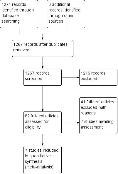
Study flow diagram: 2006 search.

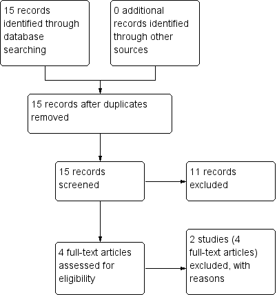
Study flow diagram: 2012 update search (no additional studies).
Study flow diagram: economic Cochrane Schizophrenia Group’s Health Economic Database (CSzGHED) search 23 July 2013.

'Risk of bias' graph: review authors' judgements about each risk of bias item presented as percentages across all included studies.

'Risk of bias' summary: review authors' judgements about each risk of bias item for each included study.

Comparison 1: ORAL FLUPHENAZINE versus PLACEBO, Outcome 1: Global state: 1. Not improved or worsened

Comparison 1: ORAL FLUPHENAZINE versus PLACEBO, Outcome 2: Global state: 2. Relapse
| Global state: 3. Percentage of time in prodrome state (skewed data) | ||||
| Study | Intervention | Mean | SD | N |
|---|---|---|---|---|
| one‐year data | ||||
| Marder 1994 | Oral fluphenazine | 10.5 | 15.90 | 17 |
| Placebo | 19.4 | 22.30 | 19 | |
| two‐year data | ||||
| Marder 1994 | Oral fluphenazine | 2.80 | 3.80 | 14 |
| Placebo | 4.90 | 5.70 | 15 | |
Comparison 1: ORAL FLUPHENAZINE versus PLACEBO, Outcome 3: Global state: 3. Percentage of time in prodrome state (skewed data)
| Global state: 4. Percentage of time in exacerbated state (skewed data) | ||||
| Study | Intervention | Mean | SD | N |
|---|---|---|---|---|
| one‐year data | ||||
| Marder 1994 | Oral fluphenazine | 11.8 | 15.00 | 17 |
| Placebo | 7.20 | 10.70 | 19 | |
| two‐year data | ||||
| Marder 1994 | Oral fluphenazine | 5.50 | 10.40 | 14 |
| Placebo | 12.9 | 13.6 | 15 | |
Comparison 1: ORAL FLUPHENAZINE versus PLACEBO, Outcome 4: Global state: 4. Percentage of time in exacerbated state (skewed data)

Comparison 1: ORAL FLUPHENAZINE versus PLACEBO, Outcome 5: Global state: 5. average score: CGI ‐ severity of illness score (high = poor)

Comparison 1: ORAL FLUPHENAZINE versus PLACEBO, Outcome 6: Leaving the study early: 1. Non‐specific reasons

Comparison 1: ORAL FLUPHENAZINE versus PLACEBO, Outcome 7: Leaving the study early: 2. Specific reason ‐ short term

Comparison 1: ORAL FLUPHENAZINE versus PLACEBO, Outcome 8: Leaving the study early: 3. Marked improvement/ hospital discharge

Comparison 1: ORAL FLUPHENAZINE versus PLACEBO, Outcome 9: Adverse effects: 1. Anticholinergic effects ‐ short term

Comparison 1: ORAL FLUPHENAZINE versus PLACEBO, Outcome 10: Adverse effects: 2. Cardivascular effects ‐ short term

Comparison 1: ORAL FLUPHENAZINE versus PLACEBO, Outcome 11: Adverse effects: 3. CNS ‐ short term

Comparison 1: ORAL FLUPHENAZINE versus PLACEBO, Outcome 12: Adverse effects: 4. Death ‐ long term

Comparison 1: ORAL FLUPHENAZINE versus PLACEBO, Outcome 13: Adverse effects: 5. Endocrine ‐ short term

Comparison 1: ORAL FLUPHENAZINE versus PLACEBO, Outcome 14: Adverse effects: 6a. Extrapyramidal effects ‐ short term

Comparison 1: ORAL FLUPHENAZINE versus PLACEBO, Outcome 15: Adverse effects: 6b. Extrapyramidal effects ‐ medium term

Comparison 1: ORAL FLUPHENAZINE versus PLACEBO, Outcome 16: Adverse effects: 7. Others ‐ short term

Comparison 1: ORAL FLUPHENAZINE versus PLACEBO, Outcome 17: Sensitivity analysis: 1. CHRONIC versus ACUTE

Comparison 1: ORAL FLUPHENAZINE versus PLACEBO, Outcome 18: Sensitivity analysis: 2. LOW DOSES (1‐5 mg/day) versus HIGH DOSES (5mg/day>)

Comparison 1: ORAL FLUPHENAZINE versus PLACEBO, Outcome 19: Sensitivity analysis: 3. OPERATIONAL CRITERIA versus LOOSE DEFINITIONS

Comparison 1: ORAL FLUPHENAZINE versus PLACEBO, Outcome 20: Sensitivity analysis: 4. BEFORE 1990 versus AFTER 1990
| ORAL FLUPHENAZINE versus PLACEBO for Schizophrenia | ||||||
| Patient or population: patients with Schizophrenia | ||||||
| Outcomes | Illustrative comparative risks* (95% CI) | Relative effect | No of Participants | Quality of the evidence | Comments | |
|---|---|---|---|---|---|---|
| Assumed risk | Corresponding risk | |||||
| Control | ORAL FLUPHENAZINE versus PLACEBO | |||||
| Global state: Not improved or worsened ‐ medium term | 680 per 10001 | 762 per 1000 | RR 1.12 | 50 | ⊕⊝⊝⊝ | |
| Global state: Relapse ‐ long term | Low | RR 0.39 | 86 | ⊕⊝⊝⊝ | Note: high degree of heterogeneity between included studies. | |
| 200 per 10001,4 | 78 per 1000 | |||||
| Moderate | ||||||
| 600 per 10001,4 | 234 per 1000 | |||||
| High | ||||||
| 800 per 10001,4 | 312 per 1000 | |||||
| Adverse effects: Death ‐ long term | Low7 | RR 2.38 | 50 | ⊕⊕⊝⊝ | ||
| 0 per 1000 | 0 per 1000 | |||||
| Moderate7 | ||||||
| 30 per 1000 | 71 per 1000 | |||||
| High7 | ||||||
| 90 per 1000 | 214 per 1000 | |||||
| Adverse effects: Extrapyramidal effects (akathisia) ‐ short term | Low8 | RR 3.43 | 227 | ⊕⊕⊕⊝ | ||
| 0 per 1000 | 0 per 1000 | |||||
| Moderate8 | ||||||
| 100 per 1000 | 343 per 1000 | |||||
| High8 | ||||||
| 200 per 1000 | 686 per 1000 | |||||
| Adverse effects: Extrapyramidal effects (rigidity) ‐ short term | Low10 | RR 3.54 | 227 | ⊕⊕⊕⊝ | ||
| 50 per 1000 | 177 per 1000 | |||||
| Moderate10 | ||||||
| 250 per 1000 | 885 per 1000 | |||||
| High10 | ||||||
| 500 per 1000 | 1000 per 1000 | |||||
| *The basis for the assumed risk (e.g. the median control group risk across studies) is provided in footnotes. The corresponding risk (and its 95% confidence interval) is based on the assumed risk in the comparison group and the relative effect of the intervention (and its 95% CI). | ||||||
| GRADE Working Group grades of evidence | ||||||
| 1 Mean baseline risk presented for single study. Key: High quality ‐ no downgrading of the evidence. | ||||||
| Study | Country | Participants | Perspective | Type of Economic Evaluation | Resource Use provided | Unit Costs Provided | ICER | QALY/DALY | Net Benefit Ratio | Grading |
|---|---|---|---|---|---|---|---|---|---|---|
| Study ID | Status | Reasons for exclusion |
|---|---|---|
| Excluded | Allocation: randomised (current systematic review). | |
| Excluded | Allocation: randomised. Particiapants: schizophrenia. Interventions: fluphenazine IM. |
| Base Case | Cost per day (£) | Cost of actual relapse (£) | Cost of relapse for study population (£)** | ||
|---|---|---|---|---|---|
| Fluphenazine | Placebo | Fluphenazine | Placebo | ||
| Median length1 of stay and mean cost2 | 5,408 | 91,936 | 205,504 | 1,437 | 3,425 |
| 116 days. | |||||
| Sensitivity analyses | Cost per day (£) | Cost of actual relapse (£) | Cost of relapse for study population (£)** | ||
|---|---|---|---|---|---|
| Fluphenazine | Placebo | Fluphenazine | Placebo | ||
| Mean length of stay1 and mean cost3 | 18,049 | 306,833 | 685,862 | 4,794 | 11,431 |
| Mean length of stay1 and mean lower quartile cost4 | 15,966 | 271,422 | 606,708 | 4,241 | 10,112 |
| Mean length of stay1 and mean upper quartile cost5 | 20,078 | 341,326 | 762,964 | 5,333 | 12,716 |
| Median length of stay2 and mean lower quartile cost4 | 4,784 | 81,328 | 181,792 | 1,271 | 3,030 |
| Median length of stay2 and mean upper quartile cost5 | 6,016 | 102,272 | 228,608 | 1,598 | 3,810 |
| 153.4 days | |||||
| Outcome or subgroup title | No. of studies | No. of participants | Statistical method | Effect size |
| 1.1 Global state: 1. Not improved or worsened Show forest plot | 3 | Risk Ratio (M‐H, Fixed, 95% CI) | Subtotals only | |
| 1.1.1 short term (CGI/MDRS) | 3 | 125 | Risk Ratio (M‐H, Fixed, 95% CI) | 0.80 [0.57, 1.12] |
| 1.1.2 medium term (MDRS) | 1 | 50 | Risk Ratio (M‐H, Fixed, 95% CI) | 1.12 [0.79, 1.58] |
| 1.2 Global state: 2. Relapse Show forest plot | 3 | 124 | Risk Ratio (M‐H, Random, 95% CI) | 0.35 [0.07, 1.68] |
| 1.2.1 short term | 1 | 38 | Risk Ratio (M‐H, Random, 95% CI) | 0.25 [0.06, 1.03] |
| 1.2.2 long term | 2 | 86 | Risk Ratio (M‐H, Random, 95% CI) | 0.39 [0.05, 3.31] |
| 1.3 Global state: 3. Percentage of time in prodrome state (skewed data) Show forest plot | 1 | Other data | No numeric data | |
| 1.3.1 one‐year data | 1 | Other data | No numeric data | |
| 1.3.2 two‐year data | 1 | Other data | No numeric data | |
| 1.4 Global state: 4. Percentage of time in exacerbated state (skewed data) Show forest plot | 1 | Other data | No numeric data | |
| 1.4.1 one‐year data | 1 | Other data | No numeric data | |
| 1.4.2 two‐year data | 1 | Other data | No numeric data | |
| 1.5 Global state: 5. average score: CGI ‐ severity of illness score (high = poor) Show forest plot | 1 | Mean Difference (IV, Fixed, 95% CI) | Subtotals only | |
| 1.5.1 short term | 1 | 36 | Mean Difference (IV, Fixed, 95% CI) | ‐0.77 [‐1.39, ‐0.15] |
| 1.6 Leaving the study early: 1. Non‐specific reasons Show forest plot | 5 | 363 | Risk Ratio (M‐H, Fixed, 95% CI) | 0.73 [0.49, 1.10] |
| 1.6.1 short term | 2 | 227 | Risk Ratio (M‐H, Fixed, 95% CI) | 0.68 [0.43, 1.07] |
| 1.6.2 medium term | 1 | 50 | Risk Ratio (M‐H, Fixed, 95% CI) | 5.00 [0.25, 99.16] |
| 1.6.3 long term | 2 | 86 | Risk Ratio (M‐H, Fixed, 95% CI) | 0.69 [0.24, 1.97] |
| 1.7 Leaving the study early: 2. Specific reason ‐ short term Show forest plot | 3 | Risk Ratio (M‐H, Fixed, 95% CI) | Subtotals only | |
| 1.7.1 administrative/hospital transfer | 1 | 37 | Risk Ratio (M‐H, Fixed, 95% CI) | 1.06 [0.07, 15.64] |
| 1.7.2 AWOL | 1 | 37 | Risk Ratio (M‐H, Fixed, 95% CI) | 1.06 [0.07, 15.64] |
| 1.7.3 court cases, transfer, eloped | 1 | 190 | Risk Ratio (M‐H, Fixed, 95% CI) | 10.65 [1.39, 81.58] |
| 1.7.4 incorrect diagnosis | 1 | 190 | Risk Ratio (M‐H, Fixed, 95% CI) | 1.07 [0.07, 16.78] |
| 1.7.5 marked early remission | 1 | 190 | Risk Ratio (M‐H, Fixed, 95% CI) | 2.13 [0.20, 23.10] |
| 1.7.6 serious complication of treatment | 1 | 190 | Risk Ratio (M‐H, Fixed, 95% CI) | 11.71 [0.66, 208.85] |
| 1.7.7 severe extrapyramidal effects | 1 | 50 | Risk Ratio (M‐H, Fixed, 95% CI) | 3.00 [0.13, 70.30] |
| 1.7.8 treatment failure | 1 | 190 | Risk Ratio (M‐H, Fixed, 95% CI) | 0.11 [0.03, 0.35] |
| 1.8 Leaving the study early: 3. Marked improvement/ hospital discharge Show forest plot | 1 | Risk Ratio (M‐H, Fixed, 95% CI) | Subtotals only | |
| 1.8.1 discharged due to marked improvement | 1 | 36 | Risk Ratio (M‐H, Fixed, 95% CI) | 3.00 [0.13, 69.09] |
| 1.9 Adverse effects: 1. Anticholinergic effects ‐ short term Show forest plot | 2 | Risk Ratio (M‐H, Fixed, 95% CI) | Subtotals only | |
| 1.9.1 blurred vision | 1 | 37 | Risk Ratio (M‐H, Fixed, 95% CI) | 5.26 [0.27, 102.66] |
| 1.9.2 constipation | 1 | 190 | Risk Ratio (M‐H, Fixed, 95% CI) | 2.22 [1.19, 4.15] |
| 1.9.3 drooling | 1 | 37 | Risk Ratio (M‐H, Fixed, 95% CI) | 3.16 [0.14, 72.84] |
| 1.9.4 dryness mouth or throat | 2 | 227 | Risk Ratio (M‐H, Fixed, 95% CI) | 3.62 [1.39, 9.42] |
| 1.9.5 gastrointestinal distress and nausea | 2 | 227 | Risk Ratio (M‐H, Fixed, 95% CI) | 0.90 [0.30, 2.72] |
| 1.9.6 increased salivation | 1 | 190 | Risk Ratio (M‐H, Fixed, 95% CI) | 18.10 [1.06, 309.15] |
| 1.9.7 nasal congestion | 1 | 37 | Risk Ratio (M‐H, Fixed, 95% CI) | 3.16 [0.14, 72.84] |
| 1.9.8 urinary disturbance | 1 | 190 | Risk Ratio (M‐H, Fixed, 95% CI) | 3.20 [0.34, 30.17] |
| 1.9.9 vomiting | 1 | 190 | Risk Ratio (M‐H, Fixed, 95% CI) | 5.32 [0.26, 109.41] |
| 1.10 Adverse effects: 2. Cardivascular effects ‐ short term Show forest plot | 2 | Risk Ratio (M‐H, Fixed, 95% CI) | Subtotals only | |
| 1.10.1 dizziness, faintness, weakness | 1 | 190 | Risk Ratio (M‐H, Fixed, 95% CI) | 2.34 [0.85, 6.49] |
| 1.10.2 hypotension | 1 | 37 | Risk Ratio (M‐H, Fixed, 95% CI) | 3.16 [0.14, 72.84] |
| 1.10.3 syncope | 1 | 37 | Risk Ratio (M‐H, Fixed, 95% CI) | 3.16 [0.14, 72.84] |
| 1.10.4 tachycardia | 1 | 37 | Risk Ratio (M‐H, Fixed, 95% CI) | 3.16 [0.14, 72.84] |
| 1.11 Adverse effects: 3. CNS ‐ short term Show forest plot | 2 | Risk Ratio (M‐H, Fixed, 95% CI) | Subtotals only | |
| 1.11.1 anxiety, agitation, excitement and confusion | 1 | 37 | Risk Ratio (M‐H, Fixed, 95% CI) | 1.06 [0.17, 6.72] |
| 1.11.2 convulsion or seizures | 1 | 190 | Risk Ratio (M‐H, Fixed, 95% CI) | 0.35 [0.01, 8.60] |
| 1.11.3 depression | 1 | 37 | Risk Ratio (M‐H, Fixed, 95% CI) | 0.35 [0.02, 8.09] |
| 1.11.4 drowsiness | 1 | 190 | Risk Ratio (M‐H, Fixed, 95% CI) | 3.91 [1.98, 7.71] |
| 1.11.5 headache | 1 | 190 | Risk Ratio (M‐H, Fixed, 95% CI) | 1.17 [0.52, 2.63] |
| 1.11.6 sedation and lethargy | 1 | 37 | Risk Ratio (M‐H, Fixed, 95% CI) | 1.06 [0.31, 3.60] |
| 1.12 Adverse effects: 4. Death ‐ long term Show forest plot | 1 | 50 | Risk Ratio (M‐H, Fixed, 95% CI) | 2.38 [0.10, 55.72] |
| 1.13 Adverse effects: 5. Endocrine ‐ short term Show forest plot | 1 | Risk Ratio (M‐H, Fixed, 95% CI) | Subtotals only | |
| 1.13.1 amenorrhea | 1 | 190 | Risk Ratio (M‐H, Fixed, 95% CI) | 1.07 [0.27, 4.14] |
| 1.13.2 lactation | 1 | 190 | Risk Ratio (M‐H, Fixed, 95% CI) | 7.45 [0.39, 142.32] |
| 1.13.3 swelling of breasts | 1 | 190 | Risk Ratio (M‐H, Fixed, 95% CI) | 5.32 [0.26, 109.41] |
| 1.14 Adverse effects: 6a. Extrapyramidal effects ‐ short term Show forest plot | 2 | Risk Ratio (M‐H, Fixed, 95% CI) | Subtotals only | |
| 1.14.1 akinesia | 1 | 37 | Risk Ratio (M‐H, Fixed, 95% CI) | 3.16 [0.14, 72.84] |
| 1.14.2 akathisia | 2 | 227 | Risk Ratio (M‐H, Fixed, 95% CI) | 3.43 [1.23, 9.56] |
| 1.14.3 associated movements | 1 | 37 | Risk Ratio (M‐H, Fixed, 95% CI) | 7.37 [0.41, 133.37] |
| 1.14.4 dystonia | 1 | 190 | Risk Ratio (M‐H, Fixed, 95% CI) | 13.84 [0.79, 242.25] |
| 1.14.5 facial rigidity | 1 | 190 | Risk Ratio (M‐H, Fixed, 95% CI) | 2.77 [1.03, 7.46] |
| 1.14.6 loss of associated movements | 1 | 190 | Risk Ratio (M‐H, Fixed, 95% CI) | 6.39 [1.95, 20.98] |
| 1.14.7 restlessness, insomnia | 2 | 227 | Risk Ratio (M‐H, Fixed, 95% CI) | 0.99 [0.69, 1.40] |
| 1.14.8 rigidity | 2 | 227 | Risk Ratio (M‐H, Fixed, 95% CI) | 3.54 [1.76, 7.14] |
| 1.14.9 tremor | 2 | 227 | Risk Ratio (M‐H, Fixed, 95% CI) | 3.19 [1.25, 8.11] |
| 1.15 Adverse effects: 6b. Extrapyramidal effects ‐ medium term Show forest plot | 1 | Risk Ratio (M‐H, Fixed, 95% CI) | Subtotals only | |
| 1.15.1 akathisia | 1 | 50 | Risk Ratio (M‐H, Fixed, 95% CI) | 1.20 [0.42, 3.43] |
| 1.15.2 akinesia | 1 | 50 | Risk Ratio (M‐H, Fixed, 95% CI) | 11.00 [0.64, 188.95] |
| 1.15.3 dystonia | 1 | 50 | Risk Ratio (M‐H, Fixed, 95% CI) | 1.09 [0.92, 1.29] |
| 1.15.4 parkinsonism | 1 | 50 | Risk Ratio (M‐H, Fixed, 95% CI) | 5.50 [1.36, 22.32] |
| 1.16 Adverse effects: 7. Others ‐ short term Show forest plot | 2 | Risk Ratio (M‐H, Fixed, 95% CI) | Subtotals only | |
| 1.16.1 convulsion or seizures | 1 | 190 | Risk Ratio (M‐H, Fixed, 95% CI) | 0.35 [0.01, 8.60] |
| 1.16.2 diarrhoea | 1 | 190 | Risk Ratio (M‐H, Fixed, 95% CI) | 5.32 [0.26, 109.41] |
| 1.16.3 intercurrent infection | 1 | 190 | Risk Ratio (M‐H, Fixed, 95% CI) | 1.07 [0.22, 5.14] |
| 1.16.4 rash | 2 | 227 | Risk Ratio (M‐H, Fixed, 95% CI) | 0.76 [0.15, 3.78] |
| 1.17 Sensitivity analysis: 1. CHRONIC versus ACUTE Show forest plot | 2 | Risk Ratio (M‐H, Fixed, 95% CI) | Subtotals only | |
| 1.17.1 Acute: Global state ‐ not improved ‐ short term | 1 | 37 | Risk Ratio (M‐H, Fixed, 95% CI) | 0.59 [0.24, 1.42] |
| 1.17.2 Chronic: global state ‐ not improved ‐ short term | 1 | 50 | Risk Ratio (M‐H, Fixed, 95% CI) | 0.93 [0.56, 1.55] |
| 1.18 Sensitivity analysis: 2. LOW DOSES (1‐5 mg/day) versus HIGH DOSES (5mg/day>) Show forest plot | 3 | Risk Ratio (M‐H, Fixed, 95% CI) | Subtotals only | |
| 1.18.1 High dose: Global state ‐ not improved ‐ short term | 1 | 38 | Risk Ratio (M‐H, Fixed, 95% CI) | 0.79 [0.48, 1.31] |
| 1.18.2 Flexible dose: Global state ‐ not improved ‐ short term | 2 | 87 | Risk Ratio (M‐H, Fixed, 95% CI) | 0.80 [0.51, 1.25] |
| 1.19 Sensitivity analysis: 3. OPERATIONAL CRITERIA versus LOOSE DEFINITIONS Show forest plot | 3 | Risk Ratio (M‐H, Fixed, 95% CI) | Subtotals only | |
| 1.19.1 DSM‐III‐R: Global state ‐ not improved ‐ short term | 1 | 38 | Risk Ratio (M‐H, Fixed, 95% CI) | 0.79 [0.48, 1.31] |
| 1.19.2 Loose definition: global state ‐ not improved ‐ short term | 2 | 87 | Risk Ratio (M‐H, Fixed, 95% CI) | 0.80 [0.51, 1.25] |
| 1.20 Sensitivity analysis: 4. BEFORE 1990 versus AFTER 1990 Show forest plot | 3 | Risk Ratio (M‐H, Fixed, 95% CI) | Subtotals only | |
| 1.20.1 Before 1990: Global state ‐ not improved ‐ short term | 2 | 87 | Risk Ratio (M‐H, Fixed, 95% CI) | 0.80 [0.51, 1.25] |
| 1.20.2 After 1990: Global state ‐ not improved ‐ short term | 1 | 38 | Risk Ratio (M‐H, Fixed, 95% CI) | 0.79 [0.48, 1.31] |