Controlled ovarian stimulation protocols for assisted reproduction: a network meta‐analysis
Abstract
This is a protocol for a Cochrane Review (Intervention). The objectives are as follows:
We aim to assess the clinical effectiveness and safety profile of currently applied controlled ovarian stimulation (COS) protocols, and to generate a clinically‐useful ranking of these protocols.
Background
Description of the condition
Infertility is common and the global burden remains high over the years (Mascarenhas 2012). The National Institute for Health and Care Excellence (NICE) recommends in‐vitro fertilisation (IVF) as the definitive treatment for prolonged unresolved infertility after other treatments have failed. IVF may be used to overcome female or male fertility problems (NICE 2013). In 2012, the number of babies born as a result of assisted reproduction technologies (ART) exceeded an estimated total of 5 million, and around 1.5 million cycles are now performed each year globally, with this number continuing to rise (ESHRE 2012). However, the success of IVF depends in part on obtaining a sufficient number of eggs to create high‐quality embryos for uterine transfer, without exposing the patient to the risks of excessive ovarian stimulation (Macklon 2006; Sunkara 2011).
Description of the intervention
Controlled ovarian stimulation (COS) comprises three basic elements.
-
Exogenous gonadotrophins to stimulate multi‐follicular development.
-
Cotreatment with either gonadotropin‐releasing hormone (GnRH) agonist or antagonists to suppress pituitary function and prevent premature ovulation.
-
Triggering of final oocyte maturation 36 to 38 hours prior to oocyte retrieval.
Gonadotrophin preparations available for use include human menopausal gonadotrophin (hMG), a urinary product with follicle‐stimulating hormone (FSH) and luteinizing hormone (LH) activity, purified FSH (p‐FSH) and highly purified FSH (hp‐FSH), and various recombinant FSH (rFSH) and LH (rFSH/rLH) preparations. In addition, IVF in an unstimulated cycle with the anticipation of only collecting a mature single egg is offered by some clinics, but this practice is not widely established.
GnRH agonists or antagonists have been used in a number of different protocols. In the so‐called 'long protocol', the GnRH agonist is started at least two weeks before stimulation and continued up until oocyte maturation is achieved. Alternatively, a 'short protocol' is used in which the GnRH agonist is commenced simultaneously with stimulation and continued up until the day of oocyte maturation trigger. Yet another option is the use of GnRH antagonists. These involve a shorter duration of use compared with the agonist 'long protocol' and are started a few days after initiation of stimulation, continuing up until administration of a drug to trigger oocyte maturation.
At the end of the stimulation phase of an IVF cycle, a drug is used to trigger the final oocyte maturation, which is used to mimic the natural endogenous LH surge and initiate the process of ovulation before the mature eggs are collected from the woman and fertilised with sperm in the laboratory. Two drugs are currently used: human chorionic gonadotropin (HCG), which is the most common drug, or GnRH agonist in an antagonist protocol.
How the intervention might work
Complex endocrine changes happen while a woman undergoes ovarian stimulation as part of IVF treatment. The two main aims of COS are: (a) to create a cohort of developing follicles; and (b) to prevent premature spontaneous ovulation.
GnRH agonists are administered intramuscularly, subcutaneously or intranasally. In the 'long protocol', the initial flare effect of the GnRH agonists is followed by desensitisation and down‐regulation of the pituitary gland with an internalisation of the GnRH receptors. This protocol is associated with a higher oocyte number and clinical pregnancy rates, but there is evidence of an increase in the requirement of gonadotrophins compared to a 'short protocol' (Siristatidis 2015).
GnRH antagonists act by binding to the GnRH receptors and prevent endogenous release of GnRH from the pituitary gland. GnRH antagonist protocols are associated with immediate LH suppression and decreased gonadotrophin use. As a result, antagonist protocols are associated with a significant reduction in ovarian hyperstimulation syndrome (OHSS) without reducing significantly the live birth rate (Al‐Inany 2016).
Triggering the final oocyte maturation with GnRH agonist in an antagonist protocol has the added advantage of reducing the incidence of OHSS further compared to HCG because of its sustained luteotrophic effect. However, live birth and ongoing pregnancy rates are lower and this is thought to be a consequence of the luteal phase defect. Modifying the luteal phase support protocols to include small dosages of HCG can increase pregnancy rates, but also increases the risk of OHSS (Humaidan 2011).
Why it is important to do this review
Since the introduction of COS for IVF, many trials have compared different regimens. There are eight separate Cochrane reviews (Al‐Inany 2016; Albuquerque 2013; Gibreel 2012; Mochtar 2007; Pouwer 2012; Siristatidis 2015; Smulders 2010; Van Wely 2011) including an aggregate total of over 200 trials and 40,000 participants, that have compared one COS protocol to another. There are, however, limitations to the currently‐available analyses. Existing Cochrane reviews have only been able to conduct head‐to‐head comparisons of two interventions at a time (direct evidence). This approach precludes evaluation of the large amount of the indirect evidence available, and in the absence of a single randomised controlled trial (RCT) comparing all available protocols, uncertainty remains over their relative effectiveness and ranking.
For a complex process such as COS with multiple possible treatment options, not all of which have been directly compared, a network meta‐analysis may be better able to allow for comparisons and conclusions about which protocol is most effective. A network meta‐analysis simultaneously pools all the available direct and indirect evidence on relative treatment effects, to achieve a single coherent analysis. Indirect evidence is obtained by inferring the relative effectiveness of two competing treatments through a common comparator (Caldwell 2005; Caldwell 2010). Thus a network meta‐analysis produces estimates of the relative effects of each treatment compared with every other in a network, even though some pairs may not have been directly compared, and has the potential to reduce the uncertainty in treatment effect estimates. It also allows for the calculation of the probability that each protocol is the best for any given outcome through a Markov chain Monte Carlo simulation. Network meta‐analysis can additionally be used to identify gaps in the evidence base for designing a future trial that will reduce the uncertainty in the treatment effect estimates.
Objectives
We aim to assess the clinical effectiveness and safety profile of currently applied controlled ovarian stimulation (COS) protocols, and to generate a clinically‐useful ranking of these protocols.
Methods
Criteria for considering studies for this review
Types of studies
We will include all randomised controlled comparisons or cluster trials that study the relative effectiveness or side‐effects of COS protocols. We will exclude cross‐over, quasi‐randomised and non‐randomised trials.
Types of participants
The review will consider trials that include women undergoing COS during IVF and intracytoplasmic sperm injection (ICSI) treatment. Trials using gonadotrophins for ovulation induction that do not involve IVF, and studies using anti‐oestrogens or aromatase inhibitors alone without gonadotropins, will be excluded. We will include all women regardless of age or expected response to the COS protocol.
Types of interventions
We will include trials comparing at least two COS protocols that use GnRH agonists or antagonists for pituitary suppression and hMG, purified urinary FSH (U‐FSH), or recombinant FSH (rFSH) with or without LH (rFSH/rLH) gonadotrophin preparations for ovarian stimulation. For poor responders we will also include trials comparing a COS protocol to a natural cycle protocol.
From the relevant Cochrane reviews we have identified at least 12 COS protocols for predicted normal/hyper‐responders and 17 COS protocols for predicted poor responders with multiple comparisons as depicted in the following network diagrams.
Figure 1 and Figure 2 show the overall network of suggested eligible comparisons in the review at a protocol level for normal/hyper‐responders and poor responders respectively. Directly comparable treatments are linked with a line. Table 1 below lists the available protocols used in the network diagrams for over‐/normal responders (Figure 1).

Graphic representation of available trials and comparisons of controlled ovarian stimulation protocols for normal/hyper‐responders.
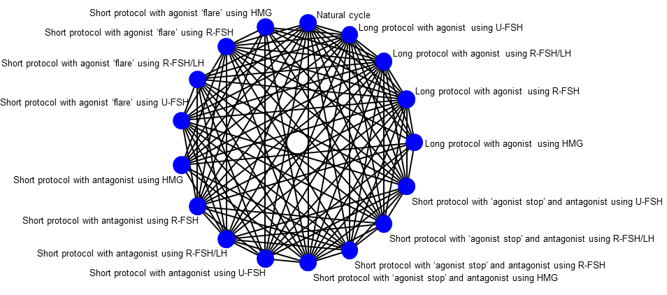
Graphic representation of available trials and comparisons of controlled ovarian stimulation protocols for poor responders.
Table 1
| Long protocol with agonist using HMG |
| Short protocol with antagonist using HMG |
| Short protocol with agonist ‘flare’ using HMG |
| Long protocol with agonist using U‐FSH |
| Short protocol with antagonist using U‐FSH |
| Short protocol with agonist ‘flare’ using U‐FSH |
| Long protocol with agonist using R‐FSH |
| Short protocol with antagonist using R‐FSH |
| Short protocol with agonist ‘flare’ using R‐FSH |
| Long protocol with agonist using R‐FSH/LH |
| Short protocol with antagonist using R‐FSH/LH |
| Short protocol with agonist ‘flare’ using R‐FSH/LH |
Table 2 below lists the available protocols included in the network diagram for poor responders (Figure 2).
Table 2
| Long protocol with agonist using HMG |
| Short protocol with antagonist using HMG |
| Short protocol with agonist ‘flare’ using HMG |
| Short protocol with ‘agonist stop’ using HMG |
| Long protocol with agonist using U‐FSH |
| Short protocol with antagonist using U‐FSH |
| Short protocol with agonist ‘flare’ using U‐FSH |
| Short protocol with ‘agonist stop’ using U‐FSH |
| Long protocol with agonist using R‐FSH |
| Short protocol with antagonist using R‐FSH |
| Short protocol with agonist ‘flare’ using R‐FSH |
| Short protocol with ‘agonist stop’ using R‐FSH |
| Long protocol with agonist using R‐FSH/LH |
| Short protocol with antagonist using R‐FSH/LH |
| Short protocol with agonist ‘flare’ using R‐FSH/LH |
| Short protocol with ‘agonist stop’ using R‐FSH/LH |
| Natural cycle |
If we identify any other protocols in the included studies we will consider them as eligible and include them in the network analyses after assessing their comparability with those named above. We plan additional analyses by grouping of the interventions (merging of GnRH agonist protocols versus GnRH antagonists or urinary FSH versus recombinant FSH or 'long' versus 'short' protocol) to investigate further class effects.
We will exclude trials that compare exclusively different dosages, regimens or routes of administration of the same drug and protocol.
Types of outcome measures
These outcomes are likely to be the most clinically‐important and commonly‐reported events in the studies that are of relevance.
All primary and secondary outcomes are calculated per woman randomised.
Primary outcomes
1. Live birth.
2. Number of women experiencing OHSS events as defined by the trialists.
Secondary outcomes
3. Clinical pregnancy, defined as evidence of a gestational sac, confirmed by ultrasound.
4. Ongoing pregnancy, defined as evidence of a gestational sac with fetal heart motion, confirmed with ultrasound.
5. Number of oocytes retrieved.
6. Multiple pregnancy rate, counted as one live birth event.
7. Miscarriage rate.
8. Ectopic pregnancy rate.
9. Cycle cancellation (defined as cancelled cycle before oocyte retrieval).
Search methods for identification of studies
No language or date restrictions will be applied.
Electronic searches
We will search the following electronic databases, trial registers and websites in consultation with the Cochrane Gynaecology and Fertility Group (CGF) Information Specialist:
-
the Gynaecology and Fertility Group (CGF) Specialised Register of Controlled Trials (Appendix 1);
-
the Cochrane Central Register of Controlled Trials (CENTRAL, Cochrane Library)(Appendix 2);
-
MEDLINE (Appendix 3);
-
Embase (Appendix 4); and
-
CINAHL (Appendix 5).
The MEDLINE search will be combined with the Cochrane highly sensitive search strategy for identifying randomized trials which appears in the Cochrane Handbook for Systematic Reviews of Interventions (Higgins 2011, section 6.4.11). The Embase and CINAHL searches are combined with trial filters developed by the Scottish Intercollegiate Guidelines Network (SIGN) (www.sign.ac.uk/methodology/filters.html#random).
Other electronic sources of trials will include:
-
trial registers for ongoing and registered trials:
-
www.clinicaltrials.gov (a service of the US National Institutes of Health);
-
www.who.int/trialsearch/Default.aspx (the World Health Organisation International Trials Registry Platform search portal);
-
-
the Web of Science ‐ wokinfo.com/ (another source of trials and conference abstracts);
-
OpenGrey ‐ www.opengrey.eu/ for unpublished literature from Europe;
-
LILACS and other Spanish/Portuguese databases, that can be found in the Virtual Health Library Regional Portal (VHL) ‐ regional.bvsalud.org/php/index.php?lang=en; and
-
PubMed and Google Scholar (for recent trials not yet indexed in the major databases).
Searching other resources
We will search for the full texts of relevant studies identified as abstracts. We will seek information from primary authors to investigate whether these studies meet eligibility criteria, and to obtain outcome and study data. Trials that compare at least two of the proposed protocols are eligible and we shall search for all possible comparisons. We will check the reference lists of published reviews and retrieved studies for additional trials.
Data collection and analysis
Selection of studies
After an initial screen of titles and abstracts retrieved by the search, we will retrieve the full texts of all potentially eligible studies. Two review authors will independently examine these full text articles for compliance with the inclusion criteria and select eligible studies. We will correspond with study investigators as required, to clarify study eligibility. We will resolve any disagreement through discussion or, if required, in consultation with a third person. If any reports require translation, we will describe the process used for data collection. Multiple reports of the same study will be collated under a single reference. We will compile a table of excluded studies, with details of any studies that a reader might plausibly expect to see included. We will document the selection process with a “PRISMA” flow chart.
Data extraction and management
We will design an electronic form in Microsoft Access software to extract data. For included studies, two review authors will extract the data using the agreed form. We will resolve discrepancies through discussion or, if required, we will consult a third person. We will enter data into Review Manager software (RevMan 2014) and check the data for accuracy. When information regarding study data is unclear, we will attempt to contact authors of the original reports to obtain further details.
Outcome data
From each included study we will extract: the number of participants, the age and the type of infertility, and any exclusion criteria. We will also extract: the interventions being compared, and their respective primary and secondary outcomes. All relevant arm‐level data will be extracted (e.g. number of events and number of patients for binary outcomes).
Data on potential effect modifiers
From each included study we will extract the following study, intervention and population characteristics that may act as effect modifiers.
-
Predicted response (hyper versus normal responders).
-
Age, body mass index and ethnicity.
-
Dosage, regimen, and route of drug administration.
Other data
From each included study we will extract the following additional information.
Country or countries in which the study was performed; date of publication; type of publication (full‐text publication, abstract publication, unpublished data); and trial registration reference.
Assessment of risk of bias in included studies
Two review authors will independently assess the risk of bias of each study using the criteria outlined in the Cochrane Handbook for Systematic Reviews of Interventions (Higgins 2011), and described below. We will resolve any disagreement by discussion or by involving a third assessor.
1. Random sequence generation (checking for possible selection bias)
We will describe for each included study the method used to generate the allocation sequence in sufficient detail to allow an assessment of whether it should produce comparable groups. Studies with high risk of bias for sequence generation (any non‐random process, e.g. odd or even date of birth; hospital or clinic record number) will be excluded.
We will assess the method as:
-
low risk of bias (any truly random process, e.g. random number table; computer random number generator); and
-
unclear risk of bias.
2. Allocation concealment (checking for possible selection bias)
We will describe for each included study the method used to conceal allocation to interventions prior to assignment and will assess whether intervention allocation could have been foreseen in advance of, or during assignment.
We will assess the methods as:
-
low risk of bias (e.g. telephone or central randomisation; consecutively numbered sealed opaque envelopes);
-
high risk of bias (open random allocation; unsealed or non‐opaque envelopes, alternation; date of birth); and
-
unclear risk of bias.
3.1 Blinding of participants, and personnel (checking for possible performance bias)
We will describe for each included study the methods used, if any, to blind study participants and personnel from knowledge of which intervention a participant received. We will consider that studies are at low risk of bias if they were blinded, or if we judge that the lack of blinding would be unlikely to affect results.
We will assess the methods as:
-
low, high or unclear risk of bias
3.2 Blinding of outcome assessment (checking for possible detection bias)
We will describe for each included study the methods used, if any, to blind outcome assessors from knowledge of which intervention a participant received. We will assess blinding separately for different outcomes. We will consider that studies are at low risk of bias if they blinded the outcome assessors, or if we judge that the lack of blinding would be unlikely to affect results. For example, lack of blinding of the outcome assessors is unlikely to introduce detection bias in this context with an objective outcome such as live birth and multiple pregnancy. Blinding, though, might influence outcomes for other adverse events such as OHSS events or cycle cancellations.
We will assess methods used to blind outcome assessment as:
• low, high or unclear risk of bias.
4. Incomplete outcome data (checking for possible attrition bias due to the amount, nature and handling of incomplete outcome data)
We will describe for each included study, and for each outcome or class of outcomes, the completeness of data including attrition and exclusions from the analysis. We will state whether attrition and exclusions were reported and the numbers included in the analysis at each stage (compared with the total randomised participants), reasons for attrition or exclusion where reported, and whether missing data were balanced across groups or were related to outcomes. Where sufficient information is reported, or can be supplied by the trial authors, we will re‐include missing data in the analyses which we undertake.
We will assess methods as:
-
low risk of bias (e.g. no missing outcome data; missing outcome data balanced across groups or not exceeding 10% for the primary outcomes of the review);
-
high risk of bias (e.g. numbers or reasons for missing data imbalanced across groups; ‘as treated’ analysis done with substantial departure of intervention received from that assigned at randomisation or exceeding 10% for the primary outcomes of the review); and
-
unclear risk of bias.
5. Selective reporting (checking for reporting bias)
We will take care to search for within‐trial selective reporting, such as trials failing to report obvious outcomes, or reporting them in insufficient detail to allow inclusion. We will seek published protocols and compare the outcomes between the protocol and the final published study. To resolve any discrepancies we will attempt to contact authors of the original reports to provide further details.
We will assess the methods as:
-
low risk of bias (where it is clear that all of the study’s prespecified outcomes and all expected outcomes of interest to the review have been reported);
-
high risk of bias (where not all the study’s prespecified outcomes have been reported; one or more reported primary outcomes were not prespecified; outcomes of interest are reported incompletely and so cannot be used; study fails to include results of a key outcome that would have been expected to have been reported); and
-
unclear risk of bias.
6. Other bias (checking for bias due to problems not covered by items 1 to 5 above)
We will describe for each included study any important concerns we have about other possible sources of bias.
We will assess whether each study was free of other problems that could put it at risk of bias, and rate each study as:
-
low risk of other bias;
-
high risk of other bias; or
-
unclear whether there is risk of other bias.
7. Overall risk of bias
We will make explicit judgements about whether studies are at high risk of bias, according to the criteria given in the Cochrane Handbook (Higgins 2011). With reference to items 1, 2 and 4 above, we will assess the likely magnitude and direction of the bias and whether we consider it is likely to impact on the findings. Studies will be ranked as being at low risk of bias if they have used a truly random process for the sequence generation, and adequate allocation concealment, and have little loss to follow up (less than 10%). The rest of the studies will be ranked as being at high risk of bias. We consider blinding to be less important with an objective outcome such as live birth. We also consider protocol publication in advance of the results to be an unsuitable criterion for sensitivity analyses, because protocol publication only became widespread in recent years. We will explore the impact of the level of bias through undertaking sensitivity analyses ‐ see Sensitivity analysis.
Measures of treatment effect
For dichotomous data, we will present results as a summary risk ratio with 95% confidence intervals (CIs). For continuous data, we will use the mean difference if outcomes are measured in the same way between trials. We will use the standardised mean difference to combine trials that measure the same outcome, but use different methods.
Relative treatment ranking
We will also estimate the ranking probabilities for all treatments of being at each possible rank for each intervention. Then we will obtain a treatment hierarchy using the surface under the cumulative ranking curve (SUCRA). SUCRA can also be expressed as a percentage of effectiveness or side‐effects of a treatment that would be ranked first without uncertainty. For primary outcomes, we will assess the robustness of these findings in sensitivity analysis by considering estimates of mean rank with 95% CIs.
Unit of analysis issues
The primary analysis will be per woman randomised; per pregnancy data may also be included for some outcomes (e.g. miscarriage). Data that do not allow valid analysis (e.g. 'per cycle' data) will be briefly summarised in an additional table and will not be meta‐analysed. Multiple live births (e.g. twins or triplets) will be counted as one live birth event. If studies report only 'per cycle' data, we will contact authors and request 'per woman' data. Some outcomes can only occur in women who reach clinical pregnancy (e.g. multiple pregnancy,and miscarriage). We will report all outcomes per randomised woman, as this is the unit of randomisation. Rates per clinical pregnancy may be used as the denominator for a secondary analysis, as this will help give the full picture.
Cluster‐randomised trials
We will include cluster‐randomised trials in the analyses along with individually‐randomised trials. We will adjust their sample sizes using the methods described in the Cochrane Handbook using an estimate of the intracluster correlation co‐efficient (ICC) derived from the trial (if possible), from a similar trial or from a study of a similar population. If we use ICCs from other sources, we will report this and conduct sensitivity analyses to investigate the effect of variation in the ICC. If we identify both cluster‐randomised trials and individually‐randomised trials, we plan to synthesise the relevant information. We will consider it reasonable to combine the results from both if there is little heterogeneity between the study designs and the interaction between the effect of intervention and the choice of randomisation unit is considered to be unlikely.
We will also acknowledge heterogeneity in the randomisation unit and perform a sensitivity analysis to investigate the effects of the randomisation unit.
Multi‐arm trials
Multi‐arm trials will be included and we will account for the correlation between the effect sizes in the network meta‐analysis. We will treat multi‐arm studies as multiple independent comparisons in pairwise meta‐analyses.
Dealing with missing data
For included studies, we will note levels of attrition. We will use sensitivity analysis to explore the impact of including studies with high levels of missing data in the overall assessment of treatment effect.
For all outcomes, we will carry out analyses, as far as possible, on an intention‐to‐treat basis, i.e. we will attempt to include all participants randomised to each group in the analyses, and all participants will be analysed in the group to which they were allocated, regardless of whether or not they received the allocated intervention. The denominator for each outcome in each trial will be the number randomised minus any participants whose outcomes are known to be missing.
Assessment of heterogeneity
Assessment of clinical and methodological heterogeneity
To evaluate the presence of clinical heterogeneity, we will generate descriptive statistics for trial and study population characteristics across all eligible trials that compare each pair of interventions. We will assess the presence of clinical heterogeneity within each pairwise comparison by comparing these characteristics.
Assessment of transitivity across treatment comparisons
We will assess the assumption of transitivity by comparing the distribution of potential effect modifiers across the different pairwise comparisons. In this context we expect that the transitivity assumption will hold, assuming the following.
-
The common COS protocol used to compare different protocols indirectly is similar when it appears in different comparisons (e.g. Long protocol with agonist using HMG is administered in a similar way to in Long protocol with agonist using HMG versus Short protocol with agonist ‘flare’ using HMG trials and in Long protocol with agonist using HMG versus Short protocol with antagonist using HMG trials).
-
All pairwise comparisons do not differ with respect to the distribution of effect modifiers (e.g. the design and study characteristics of Long protocol with agonist using HMG versus Short protocol with agonist ‘flare’ using HMG trials are similar to Long protocol with agonist using HMG versus Short protocol with antagonist using HMG trials).
The assumption of transitivity will be evaluated epidemiologically by comparing the clinical and methodological characteristics of sets of studies grouped by treatment comparisons.
Assessment of statistical heterogeneity and inconsistency
Assumptions when estimating heterogeneity
In standard pairwise meta‐analyses we will estimate different heterogeneity variances for each pairwise comparison. In network meta‐analysis we will assume a common estimate for the heterogeneity variance across the different comparisons.
Measures and tests for heterogeneity
We will assess statistically the presence of heterogeneity within each pairwise comparison using the I2 statistic and its 95% CI that measures the percentage of variability that cannot be attributed to random error, with an I2 statistic above 50% representing substantial heterogeneity.
The assessment of statistical heterogeneity in the entire network will be based on the magnitude of the heterogeneity variance parameter (τ2) estimated from the network meta‐analysis models. For dichotomous outcomes the magnitude of the heterogeneity variance will be compared with the empirical distribution as derived by Turner. We will also estimate a total I2 value for heterogeneity in the network as described elsewhere.
Assessment of statistical inconsistency
The statistical agreement between the various sources of evidence in a network of interventions (consistency) will be evaluated by global and local approaches to complement the evaluation of transitivity.
Local approaches for evaluating inconsistency
To evaluate the presence of inconsistency locally we will use the loop‐specific approach. This method evaluates the consistency assumption in each closed loop of the network separately as the difference between direct and indirect estimates for a specific comparison in the loop (inconsistency factor). Then, the magnitude of the inconsistency factors and their 95% CIs can be used to infer about the presence of inconsistency in each loop. We will assume a common heterogeneity estimate within each loop.
Global approaches for evaluating inconsistency
To check the assumption of consistency in the entire network we will use the ‘design‐by‐treatment’ model as described by Higgins and colleagues (Higgins 2012). This method accounts for different sources of inconsistency that can occur when studies with different designs (two‐arm trials versus three‐arm trials) give different results as well as disagreement between direct and indirect evidence. Using this approach we will infer about the presence of inconsistency from any source in the entire network based on a Chi2 test. The design‐by‐treatment model will be performed in STATA (Statacorp 2014) using the 'network' command (White 2015).
Inconsistency and heterogeneity are interweaved; to distinguish between these two sources of variability we will employ the I2 for inconsistency that measures the percentage of variability that cannot be attributed to random error or heterogeneity (within comparison variability).
Assessment of reporting biases
In view of the difficulty of detecting and correcting for publication bias and other reporting biases, we will aim to minimise their potential impact by ensuring a comprehensive search for eligible studies and by being alert for duplication of data. If there are ten or more studies in the network meta‐analysis, we will use a funnel plot to explore the possibility of small study effects (a tendency for estimates of the intervention effect to be more beneficial in smaller studies) and account for the fact that studies estimate effects for different comparisons.
Data synthesis
Methods for direct treatment comparisons
We will perform standard pairwise meta‐analyses using a random‐effects model in the presence of substantial heterogeneity, or a fixed‐effect model in STATA for every treatment contrast (Der Simonian 1986).
Methods for indirect and mixed comparisons
We will perform network meta‐analysis using a random‐effects model in STATA using the 'network' command for network meta‐analysis (White 2015) and other STATA commands for visualising and reporting results in network meta‐analysis (Chaimani 2015).
Subgroup analysis and investigation of heterogeneity
We will stratify all effects according to the predicted response (normal versus over responders as defined by the trialists). to explore subgroups that could affect comparative effectiveness. We will assess subgroup differences by interaction tests available within STATA. We will report the results of subgroup analyses quoting the Chi2 statistic and P value, and the interaction test I2 value.
If we find important heterogeneity and/or inconsistency, we will explore the possible sources. If sufficient studies are available, we will perform meta‐regression or subgroup analyses by using the following effect modifiers as possible sources of inconsistency and or heterogeneity:
-
age (≥ 35 versus < 35 years), body mass index (≥ 30 versus < 30) and ethnicity (white versus non‐white);
-
dosage, regimen, and route of drug administration;
-
agonist trigger versus hCG for antagonist protocols; and
-
mixed recombinant and purified FSH versus standard protocols.
We will assess subgroup differences by evaluating the relative effects and assessment of model fit for the primary outcomes. Multi‐arm trials that compare different dosages, regimens or routes of drug administration within one protocol, but also compare those versus another protocol, will be included. Intervention arms of different dosages, regimens or routes of the same drug will be merged together for the global analysis of all outcomes and treated as separate independent comparisons only for the relevant subgroup analysis according to dosage, regimen and route of drug administration, while taking into account the correlation between the comparisons.
Sensitivity analysis
For the primary outcomes we will perform sensitivity analysis for the following:
-
overall quality of the studies (low versus high risk of overall bias);
-
randomisation unit (cluster versus individual);
-
use of fixed‐effect versus random‐effects model; and
-
different effect measures (risk versus odds ratio).
Differences will be assessed by evaluating the relative effects and assessment of model fit.
'Summary of findings' table
We will present 'Summary of findings' tables using GRADEpro software (GRADEpro GDT 2014). We will follow the approach suggested by Puhan et al. (Puhan 2014; Schunemann 2009) and provide estimates from the network meta‐analysis. This table will evaluate the overall quality of the body of evidence for the primary review outcomes (live births and OHSS), using GRADE criteria (study limitations, consistency of effect, imprecision, indirectness and publication bias). Judgements about evidence quality (high, moderate or low) will be justified, documented, and incorporated into reporting of results for each outcome.
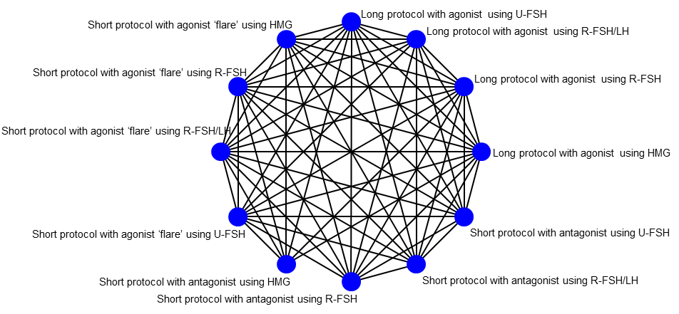
Graphic representation of available trials and comparisons of controlled ovarian stimulation protocols for normal/hyper‐responders.

Graphic representation of available trials and comparisons of controlled ovarian stimulation protocols for poor responders.