遗传性血色素沉着症的干预措施
Appendices
Appendix 1. Methods for network meta‐analysis if we find this is possible in the future
Measures of treatment effect
Relative treatment effects
For dichotomous variables (e.g. proportion of participants with serious adverse events or any adverse events), we will calculate the odds ratio with 95% credible interval (or Bayesian confidence interval) (Severini 1993). For continuous variables (e.g. quality of life reported on the same scale), we will calculate the mean difference with 95% credible interval. We will use standardised mean difference values with 95% credible interval for quality of life if included trials use different scales. For count outcomes (e.g. number of adverse events and serious adverse events), we will calculate the rate ratio with 95% credible interval. For time‐to‐event data (e.g. mortality at maximal follow‐up), we will calculate hazard ratio with 95% credible interval.
Relative ranking
We will estimate the ranking probabilities for all treatments of being at each possible rank for each intervention. Then, we will obtain the surface under the cumulative ranking curve (SUCRA) (cumulative probability) and rankogram (Salanti 2011; Chaimani 2013).
Unit of analysis issues
We will collect data for all trial treatment groups that meet the inclusion criteria. The codes for analysis, that we will use, accounts for the correlation between the effect sizes from trials with more than two groups.
Assessment of heterogeneity
We will assess clinical and methodological heterogeneity by carefully examining the characteristics and design of included trials. We will assess the presence of clinical heterogeneity by comparing effect estimates under different categories of potential effect modifiers. Different study designs and risk of bias may contribute to methodological heterogeneity.
We will assess the statistical heterogeneity by comparing the results of the fixed‐effect model meta‐analysis and the random‐effects model meta‐analysis, between‐study standard deviation (tau2 and comparing this with values reported in the study of the distribution of between‐study heterogeneity (Turner 2012)), and by calculating I2 (using Stata/SE 14.2). If we identify substantial heterogeneity, clinical, methodological, or statistical, we will explore and address heterogeneity in a subgroup analysis (see ‘Subgroup analysis and investigation of heterogeneity for network meta‐analysis’ section).
Assessment of transitivity across treatment comparisons
We will evaluate the plausibility of transitivity assumption (the assumption that the participants included in the different studies with different immunosuppressive regimens can be considered to be a part of a multi‐arm randomised clinical trial and could potentially have been randomised to any of the treatments) (Salanti 2012). In other words, any participant that meets the inclusion criteria is, in principle, equally likely to be randomised to any of the above eligible interventions. If there is any concern that the clinical safety and effectiveness are dependent upon the effect modifiers, we will continue to do traditional Cochrane pairwise comparisons and we will not perform a network meta‐analysis on all participant subgroups.
Assessment of reporting biases
For the network meta‐analysis, we will judge the reporting bias by the completeness of the search (i.e. searching various databases and including conference abstracts), as we do not currently find any meaningful order to perform a comparison‐adjusted funnel plot as suggested by Chaimani 2012. However, if we find any meaningful order, for example, the control group used depended upon the year of conduct of the trial, we will use comparison‐adjusted funnel plot as suggested by Chaimani 2012.
Data synthesis
Methods for indirect and mixed comparisons
We will conduct network meta‐analyses to compare multiple interventions simultaneously for each of the primary and secondary outcomes. Network meta‐analysis combines direct evidence within trials and indirect evidence across trials (Mills 2012). We will obtain a network plot to ensure that the trials were connected by treatments using Stata/SE 14.2 (Chaimani 2013). We will exclude any trials that were not connected to the network. We will conduct a Bayesian network meta‐analysis using the Markov chain Monte Carlo method in OpenBUGS 3.2.3 as per the guidance from the National Institute for Health and Care Excellence (NICE) Decision Support Unit (DSU) documents (Dias 2014a). We will model the treatment contrast (i.e. log odds ratio for binary outcomes, mean difference or standardised mean difference for continuous outcomes, log rate ratio for count outcomes, and log hazard ratio for time‐to‐event outcomes) for any two interventions ('functional parameters') as a function of comparisons between each individual intervention and an arbitrarily selected reference group ('basic parameters') (Lu 2006) using appropriate likelihood functions and links. We will use binomial likelihood and logit link for binary outcomes, Poisson likelihood and log link for count outcomes, binomial likelihood and complementary log‐log link for time‐to‐event outcomes, and normal likelihood and identity link for continuous outcomes. We will perform a fixed‐effect model and random‐effects model for the network meta‐analysis. We will report both models for comparison with the reference group in a forest plot. For pairwise comparison, we will report the fixed‐effect model if the two models reported similar results; otherwise, we will report the more conservative model.
We will use a hierarchical Bayesian model using three different initial values using codes provided by NICE DSU (Dias 2014a). We will use a normal distribution with large variance (10,000) for treatment effect priors (vague or flat priors). For the random‐effects model, we will use a prior distributed uniformly (limits: 0 to 5) for between‐trial standard deviation but assumed similar between‐trial standard deviation across treatment comparisons (Dias 2014a). We will use a 'burn‐in' of 5000 simulations, check for convergence visually, and run the models for another 10,000 simulations to obtain effect estimates. If we did not obtain convergence, we will increase the number of simulations for 'burn‐in'. If we do not obtain convergence still, we will use alternate initial values and priors using methods suggested by van Valkenhoef 2012. We will also estimate the probability that each intervention ranks at one of the possible positions using the NICE DSU codes (Dias 2014a).
Assessment of inconsistency
We will assess inconsistency (statistical evidence of the violation of transitivity assumption) by fitting both an inconsistency model and a consistency model. We will use the inconsistency models used in the NICE DSU manual, as we plan to use a common between‐study deviation for the comparisons (Dias 2014b). In addition, we will use the design‐by‐treatment full interaction model (Higgins 2012) and IF (inconsistency factor) plots (Chaimani 2013) to assess inconsistency. In the presence of inconsistency, we will assess whether the inconsistency is because of clinical or methodological heterogeneity by performing separate analyses for each of the different subgroups mentioned in the ‘Subgroup analysis and investigation of heterogeneity for network meta‐analysis’ section below.
If there is evidence of inconsistency, we will identify areas in the network where substantial inconsistency might be present in terms of clinical and methodological diversities between trials and, when appropriate, limit network meta‐analysis to a more compatible subset of trials.
Direct comparison
We will perform the direct comparisons using the same codes and the same technical details.
Sample size calculations
To control for the risk of random errors, we will interpret the information with caution when the accrued sample size in the network meta‐analysis (i.e. across all treatment comparisons) was less than the required sample size (required information size). For calculation of the required information size, see Appendix 3.
Subgroup analysis and investigation of heterogeneity for network meta‐analysis
We will assess the differences in the effect estimates between the subgroups listed in Subgroup analysis and investigation of heterogeneity using meta‐regression with the help of the OpenBUGS code (Dias 2012a) if we include a sufficient number of trials. We will use the potential modifiers as study level co‐variates for meta‐regression. We will calculate a single common interaction term (Dias 2012a). If the 95% credible intervals of the interaction term do not overlap zero, we will consider this as evidence of difference in subgroups.
Presentation of results
We will present the effect estimates with 95% CrI for each pairwise comparisons calculated from the direct comparisons and network meta‐analysis. We will also present the cumulative probability of the treatment ranks (i.e. the probability that the treatment is within the top two, the probability that the treatment is within the top three, etc.) in graphs (surface under the cumulative ranking curve or SUCRA) (Salanti 2011). We will also plot the probability that each treatment is best, second best, third best etc for each of the different outcomes (rankograms), which are generally considered more informative (Salanti 2011; Dias 2012b).
We will present the 'Summary of findings' tables for mortality. In the 'summary of findings Table for the main comparison', we will follow the approach suggested by Puhan et al. (Puhan 2014). First, we will calculate the direct and indirect effect estimates and 95% credible intervals using the node‐splitting approach (Dias 2010), i.e. calculate the direct estimate for each comparison by including only trials in which there was direct comparison of treatments and the indirect estimate for each comparison by excluding the trials in which there was direct comparison of treatments. Then we will rate the quality of direct and indirect effect estimates using GRADE which takes into account the risk of bias, inconsistency, directness of evidence, imprecision, and publication bias (Guyatt 2011). Then, we will present the estimates of the network meta‐analysis and rate the quality of network meta‐analysis effect estimates as the best quality of evidence between the direct and indirect estimates (Puhan 2014). In addition, in the same table, we will present illustrations and information on the number of trials and participants as per the standard 'Summary of Findings' Table.
Appendix 2. Search strategies
| Database | Time span | Search strategy |
| The Central Register of Controlled Trials (CENTRAL) (Wiley) | 2016, Issue 3 | #1 MeSH descriptor: [Hemochromatosis] explode all trees #2 (hemochromatos* or hemochromatos* or iron overload or ironoverload) #3 #1 or #2 |
| MEDLINE (OvidSP) | January 1947 to March 2016 | 1. exp Hemochromatosis/ 2. (hemochromatos* or hemochromatos* or iron overload or ironoverload).ti,ab. 3. 1 or 2 4. randomized controlled trial.pt. 5. controlled clinical trial.pt. 6. randomized.ab. 7. placebo.ab. 8. drug therapy.fs. 9. randomly.ab. 10. trial.ab. 11. groups.ab. 12. 4 or 5 or 6 or 7 or 8 or 9 or 10 or 11 13. exp animals/ not humans.sh. 14. 12 not 13 15. 3 and 14 |
| Embase (OvidSP) | January 1974 to March 2016 | 1. exp hemochromatosis/ 2. (hemochromatos* or hemochromatos* or iron overload or ironoverload).ti,ab. 3. 1 or 2 4. exp crossover‐procedure/ or exp double‐blind procedure/ or exp randomized controlled trial/ or single‐blind procedure/ 5. (((((random* or factorial* or crossover* or cross over* or cross‐over* or placebo* or double*) adj blind*) or single*) adj blind*) or assign* or allocat* or volunteer*).af. 6. 4 or 5 7. 3 and 6 |
| Science Citation Index Expanded (Web of Knowledge) | January 1945 to March 2016 | #1 TS=(hemochromatos* or hemochromatos* or iron overload or ironoverload) #2 TS=(random* OR rct* OR crossover OR masked OR blind* OR placebo* OR meta‐analysis OR systematic review* OR meta‐analys*) #3 #1 AND #2 |
| World Health Organization International Clinical Trials Registry Platform Search Portal (apps.who.int/trialsearch/Default.aspx) | March 2016 | Condition: hemochromatos* or hemochromatos* or iron overload or ironoverload |
| March 2016 | Interventional Studies | (hemochromatos* OR hemochromatos* OR iron overload OR ironoverload) | Phase 2, 3, 4 |
Appendix 3. Sample size calculation
The five‐year mortality in people with hereditary haemochromatosis is 5% (Wojcik 2002). The required information size based on a control group proportion of 20%, a relative risk reduction of 20% in the intervention group, type I error of 5%, and type II error of 20% is 13,492 participants. Network analyses are more prone to the risk of random errors than direct comparisons (Del Re 2013). Accordingly, a greater sample size is required in indirect comparisons than direct comparisons (Thorlund 2012). The power and precision in indirect comparisons depends upon various factors, such as the number of participants included under each comparison and the heterogeneity between the trials (Thorlund 2012). If there is no heterogeneity across the trials, the sample size in indirect comparisons would be equivalent to the sample size in direct comparisons. The effective indirect sample size can be calculated using the number of participants included in each direct comparison (Thorlund 2012). For example, a sample size of 2500 participants in the direct comparison A versus C (nAC) and a sample size of 7500 participants in the direct comparison B versus C (nBC) results in an effective indirect sample size of 1876 participants. However, in the presence of heterogeneity within the comparisons, the sample size required is higher. In the above scenario, for an I2 statistic for each of the comparisons A versus C (IAC2) and B versus C (IBC2) of 25%, the effective indirect sample size is 1407 participants. For an I2 statistic for each of the comparisons A versus C and B versus C of 50%, the effective indirect sample size is 938 participants (Thorlund 2012). If there were only three groups and the sample size in the trials is more than the required information size, we will calculate the effective indirect sample size using the following generic formula (Thorlund 2012):
((nAC x (1 ‐ IAC2)) x (nBC x (1 ‐ IBC2))/((nAC x (1 ‐ IAC2)) + (nBC x (1 ‐ IBC2)).
There is currently no method to calculate the effective indirect sample size for a network analysis involving more than three intervention groups.
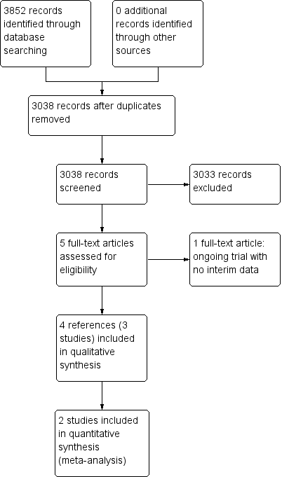
Study flow diagram.

Risk of bias graph: review authors' judgements about each risk of bias item presented as percentages across all included studies.

Risk of bias summary: review authors' judgements about each risk of bias item for each included study.
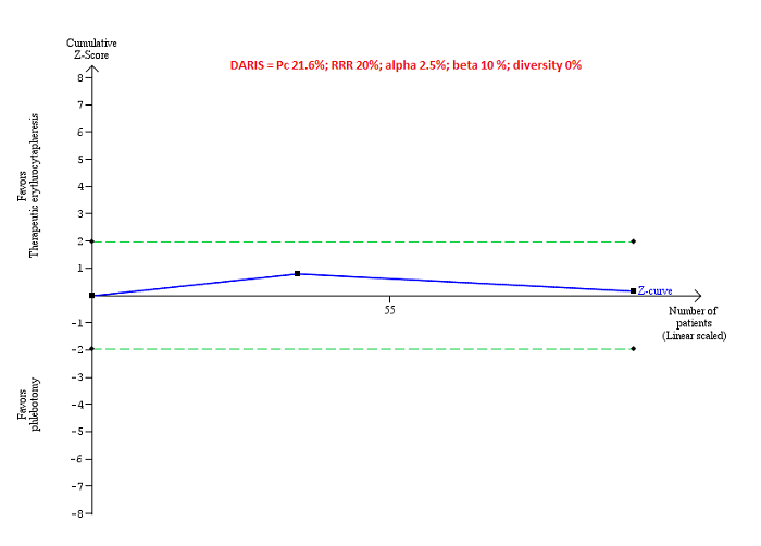
Trial Sequential Analysis of adverse events (proportion) performed using an alpha error of 2.5%, power of 90% (beta error of 10%), relative risk reduction of 20%, control group proportion (Pc) observed in trials (21.6% for proportion of people with adverse events), and observed diversity (0%) shows that the accrued sample size was only a small fraction of the diversity‐adjusted required information size (DARIS) that the boundaries could not be drawn. The Z‐curve (blue line) does not cross the conventional boundaries (dotted green line). There was a high risk of random errors.
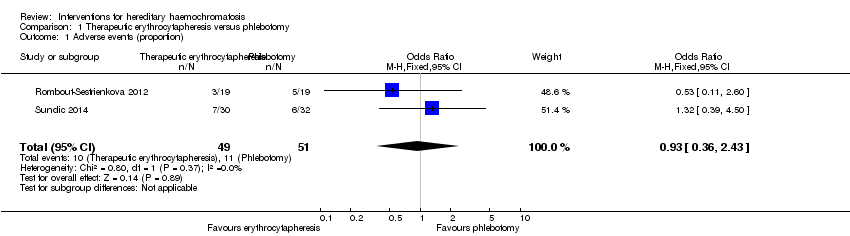
Comparison 1 Therapeutic erythrocytapheresis versus phlebotomy, Outcome 1 Adverse events (proportion).

Comparison 1 Therapeutic erythrocytapheresis versus phlebotomy, Outcome 2 Adverse events (number).

Comparison 1 Therapeutic erythrocytapheresis versus phlebotomy, Outcome 3 Health‐related quality of life (EQ‐VAS).
| Erythrocytapheresis versus phlebotomy for hereditary haemochromatosis | |||||
| Patient or population: people with hereditary haemochromatosis | |||||
| Outcomes | Illustrative comparative risks* (95% CI) | Relative effect | No of participants | Quality of the evidence | |
| Assumed risk | Corresponding risk | ||||
| Phlebotomy | Therapeutic erythrocytapheresis | ||||
| Long‐term mortality | None of the included trials reported mortality beyond 1 year. | ||||
| Mortality Follow‐up period: 8 months | There was no mortality in either group in the short‐term in the 1 trial that reported this information. | 38 | ⊕⊝⊝⊝ | ||
| Serious adverse events Follow‐up period: 8 months | There were no serious adverse events in either group in the 1 trial that reported this information. | 38 | ⊕⊝⊝⊝ | ||
| Health‐related quality of life Follow‐up period: 8 months | The mean health‐related quality of life in the control groups was | The mean health‐related quality of life in the intervention groups was | ‐ | 38 | ⊕⊝⊝⊝ |
| Health‐related quality of life beyond one year | None of the included trials reported health‐related quality of life beyond one year | ||||
| *The basis for the assumed risk is the mean control group proportion or control event rate. The corresponding risk (and its 95% confidence interval) is based on the assumed risk in the comparison group and the relative effect of the intervention (and its 95% CI). | |||||
| GRADE Working Group grades of evidence | |||||
| 1 Downgraded one level for risk of bias. | |||||
| Outcome or subgroup title | No. of studies | No. of participants | Statistical method | Effect size |
| 1 Adverse events (proportion) Show forest plot | 2 | 100 | Odds Ratio (M‐H, Fixed, 95% CI) | 0.93 [0.36, 2.43] |
| 2 Adverse events (number) Show forest plot | 1 | Rate Ratio (Fixed, 95% CI) | Totals not selected | |
| 3 Health‐related quality of life (EQ‐VAS) Show forest plot | 1 | Mean Difference (IV, Fixed, 95% CI) | Totals not selected | |