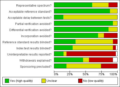
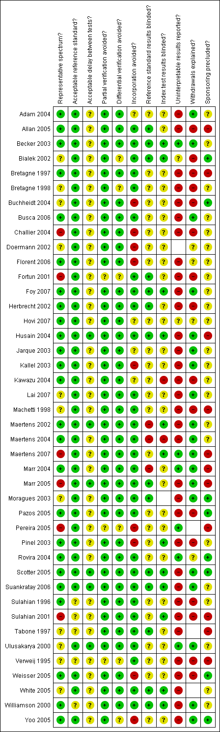
| What factors influence the diagnostic accuracy of galactomannan for invasive aspergillosis? Patients/population: immunocompromized patients, mostly hematology patients. Prior testing: varied, mostly underlying disease or symptoms (fever, neutropenia). Setting: mainly hematology or cancer departments, mainly inpatients. Index test: a sandwich ELISA for galactomannan, an Aspergillus antigen. Importance: depends on the time‐gain the test may give. Reference standard: gold standard is autopsy, but that is nearly never done; so in most studies the reference standard is composed of clinical and microbiological criteria. Studies: patient series or case‐control studies, not using an in‐house test and not excluding possibly infected patients. Studies had to report cut‐off values that were used (n = 29). The analyses were done with cut‐off value as first covariate and additional characteristics as second covariate. |
| Subgroup | Second Covariate | Sensitivity (95% CI) | Specificity (95% CI) | Comments |
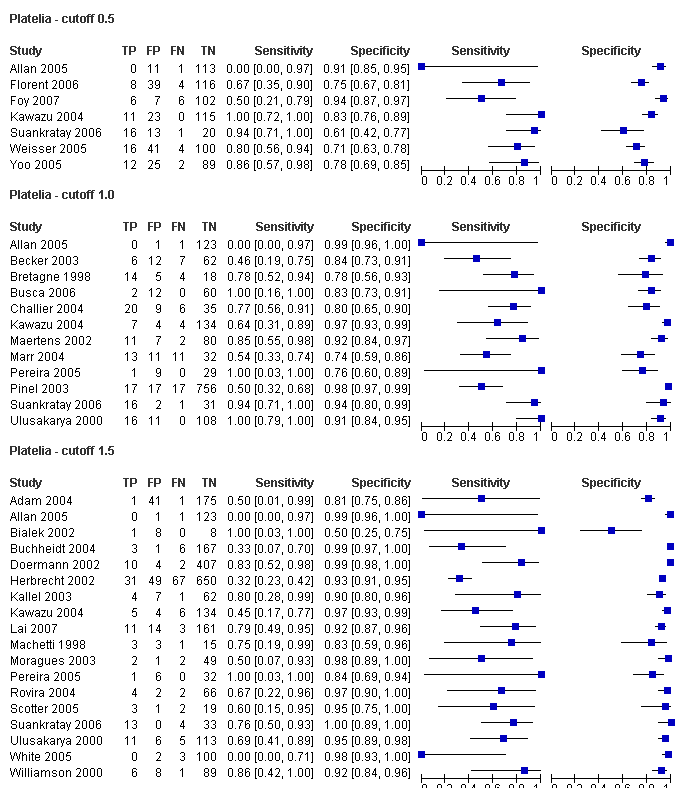
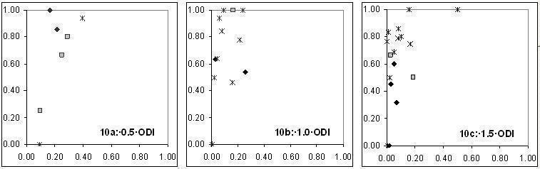
| Cut‐off 0.5 ODI | None | 0.79 (0.64 to 0.93) | 082 (0.71 to 0.92) | For none of the covariates added to cut‐off value 0.5 ODI, sensitivity or specificity exceeded 90%. The studies that selected only patients with unresponsive fever reported a significantly lower sensitivity than the other two groups (P = 0.0093). Antifungal prophylaxis significantly decreased specificity (P = 0.029). Antifungal therapy significantly increased specificity (P = 0.047). Using the EORTC criteria was associated with a significantly lower sensitivity (P = 0.03). |
| No selection Unresponsive fever Other selection | 0.73 (0.54 to 0.92) 0.68 (0.45 to 0.90) 0.89 (0.79 to 0.99) | 0.83 (0.69 to 0.96) 0.88 (0.77 to 0.99) 0.82 (0.67 to 0.96) |
| Antifungal prohylaxis No prophylaxis | 0.82 (0.69 to 0.96) 0.71 (0.51 to 0.92) | 0.88 (0.80 to 0.96) 0.77 (0.65 to 0.89) |
| Antifungal therapy No therapy | 0.82 (0.70 to 0.95) 0.64 (0.39 to 0.90) | 0.89 (0.80 to 0.98) 0.78 (0.67 to 0.90) |
| EORTC criteria used Other criteria used | 0.69 (0.52 to 0.86) 0.86 (0.76 to 0.97) | 0.85 (0.75 to 0.95) 0.82 (0.70 to 0.95) |
| Cut‐off 1.0 ODI | None | 0.71 (0.61 to 0.81) | 090 (0.87 to 0.94) | Sensitivity varies from 54% to 83%, depending on the subgroup tested. Specificity varies from 86% to 94%. The studies that selected only patients with unresponsive fever reported a significantly lower sensitivity than the other two groups (P = 0.0093). Antifungal prophylaxis significantly decreased specificity (P = 0.029). Antifungal therapy significantly increased specificity (P = 0.047). Using the EORTC criteria was associated with a significantly lower sensitivity (P = 0.03). |
| No selection Unresponsive fever Other selection | 0.61 (0.38 to 0.83) 0.54 (0.34 to 0.75) 0.82 (0.73 to 0.91) | 0.89 (0.87 to 0.98) 0.93 (0.87 to 0.99) 0.89 (0.82 to 0.95) |
| Antifungal prohylaxis No prophylaxis | 0.77 (0.64 to 0.89) 0.64 (0.47 to 0.80) | 0.93 (0.90 to 0.97) 0.86 (0.80 to 0.92) |
| Antifungal therapy No therapy | 0.76 (0.66 to 0.87) 0.56 (0.34 to 0.77) | 0.94 (0.90 to 0.98) 0.88 (0.83 to 0.93) |
| EORTC criteria used Other criteria used | 0.63 (0.51 to 0.75) 0.83 (0.73 to 0.93) | 0.90 (0.85 to 0.95) 0.88 (0.81 to 0.95) |
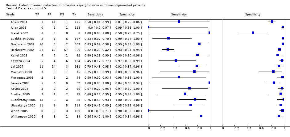
| Cut‐off 1.5 ODI | None | 0.62 (0.45 to 0.79) | 0.95 (0.92 to 0.98) | Although a cut‐off value of 1.5 ODI results in the highest specificity, sensitivity may be below 50% in some situations. The studies that selected only patients with unresponsive fever reported a significantly lower sensitivity than the other two groups (P = 0.0093). Antifungal prophylaxis significantly decreased specificity (P = 0.029). Antifungal therapy significantly increased specificity (P = 0.047). Using the EORTC criteria was associated with a significantly lower sensitivity (P = 0.03). |
| No selection Unresponsive fever Other selection | 0.47 (0.16 to 0.78) 0.40 (0.17 to 0.64) 0.72 (0.58 to 0.87) | 0.94 (0.87 to 1.00) 0.96 (0.91 to 1.00) 0.93 (0.89 to 0.97) |
| Antifungal prohylaxis No prophylaxis | 0.55 (0.34 to 0.77) 0.70 (0.51 to 0.89) | 0.96 (0.94 to 0.99) 0.92 (0.87 to 0.97) |
| Antifungal therapy No therapy | 0.69 (0.52 to 0.86) 0.46 (0.21 to 0.71) | 0.97 (0.95 to 0.99) 0.93 (0.90 to 0.97) |
| EORTC criteria used Other criteria used | 0.57 (0.40 to 0.74) 0.79 (0.65 to 0.94) | 0.93 (0.89 to 0.97) 0.92 (0.86 to 0.98) |