Información sobre normas sociales en cuanto al consumo indebido de alcohol en estudiantes universitarios
Appendices
Appendix 1. Ovid MEDLINE search strategy
Phase 1:
1. RANDOMIZED CONTROLLED TRIAL.pt.
2. CONTROLLED CLINICAL TRIAL.pt.
3. RANDOMIZED CONTROLLED TRIALS.sh.
4. RANDOM ALLOCATION. sh.
5. DOUBLE BLIND METHOD. sh.
6. SINGLE BLIND METHOD. sh.
7. or/1 6
8. ANIMALS. sh. not HUMAN. sh.
9. 7 not 8
Phase 2:
10. CLINICAL TRIAL.pt.
11. exp CLINICAL TRIALS/
12. (clin$ adj25 trial$).ti,ab.
13. ((singl$ or doubl$ or trebl$ or tripl$) adj25 (blind$ or mask$)).ti,ab.
14. PLACEBOS.sh.
15. placebo$.ti,ab.
16. random$.ti,ab.
17. RESEARCH DESIGN. sh.
18. or /10‐ 17
19. 18 not 8
20. 19 not 9
21. 9 or 20
Alcohol, social norms and student terms:
22. Brief intervention$.mp. [mp=title, subject heading word, abstract, instrumentation]
23. Social norms intervention$.mp. [mp=title, subject heading word, abstract, instrumentation]
24. (Social$ adj1 norms$).ti,ab.
25. (norm$ adj1 feedback$).ti,ab.
26. (person$ adj1 feedback$).ti,ab.
27. (individual$ adj1 feedback$).ti,ab.
28. (computer$ adj1 feedback$).ti,ab.
29. (market$ adj1 campaign$).ti,ab.
30. normative$.ti,ab.
31. or/ 22 ‐ 30
32. Alcohol$.mp. [mp=title, subject heading word, abstract, instrumentation]
33. Alcohol intervention$.mp. [mp=title, subject heading word, abstract, instrumentation]
34. (alcohol$ adj1use$).ti,ab.
35. (alcohol$ adj1 abuse$).ti,ab.
36. (alcohol$ adj1 misuse$).ti,ab.
37. (binge$ adj1 drink$).ti,ab.
38. binge drink$.mp. [mp=title, subject heading word, abstract, instrumentation]
39. alcohol use$.mp. [mp=title, subject heading word, abstract, instrumentation]
40. alcohol abuse$.mp. [mp=title, subject heading word, abstract, instrumentation]
41. alcohol misuse$.mp. [mp=title, subject heading word, abstract, instrumentation]
42. (alcohol$ adj1 problems$).ti,ab.
43. or/ 32‐42
44. Student$.mp[mp=title, subject heading word, abstract, instrumentation]
45. (university$ adj1 student$).ti,ab.
46. (college$ adj1 student$).ti,ab.
47. education$.mp[mp=title, subject heading word, abstract, instrumentation]
48. or/ 44‐47
44. 21 and 31 and 43 and 48
Appendix 2. Ovid EMBASE, CINAHL, PsycINFO search strategy
-
Brief intervention$.mp. [mp=title, abstract, subject headings, heading word, drug trade name, original title, device manufacturer, drug manufacturer name]
-
Social norms intervention$.mp. [mp=title, abstract, subject headings, heading word, drug trade name, original title, device manufacturer, drug manufacturer name]
-
(Social$ adj1 norm$).ti,ab.
-
(norm$ adj1 feedback$).ti,ab.
-
(person$ adj1 feedback$).ti,ab.
-
(individual$ adj1 feedback$).ti,ab.
-
(computer$ adj1 feedback$).ti,ab.
-
(market$ adj1 campaign$).ti,ab.
-
normative$.ti,ab.
-
or/1‐9
-
Alcohol$.mp. [mp=title, abstract, subject headings, heading word, drug trade name, original title, device manufacturer, drug manufacturer name]
-
alcohol intervention$.mp. [mp=title, abstract, subject headings, heading word, drug trade name, original title, device manufacturer, drug manufacturer name]
-
(alcohol$ adj1 use$).ti,ab.
-
(alcohol$ adj1 abuse$).ti,ab.
-
(alcohol$ adj1 misuse$).ti,ab.
-
(binge$ adj1 drink$).ti,ab.
-
binge drink$.mp. [mp=title, abstract, subject headings, heading word, drug trade name, original title, device manufacturer, drug manufacturer name]
-
alcohol use$.mp. [mp=title, abstract, subject headings, heading word, drug trade name, original title, device manufacturer, drug manufacturer name]
-
alcohol abuse$.mp. [mp=title, abstract, subject headings, heading word, drug trade name, original title, device manufacturer, drug manufacturer name]
-
alcohol misuse$.mp. [mp=title, abstract, subject headings, heading word, drug trade name, original title, device manufacturer, drug manufacturer name]
-
(alcohol$ adj1 problem$).ti,ab.
-
or/11‐21
-
10 and 22
-
student$.mp. [mp=title, abstract, subject headings, heading word, drug trade name, original title, device manufacturer, drug manufacturer name]
-
(university$ adj1 student$).ti,ab.
-
(college$ adj1 student$).ti,ab.
-
education$.mp. [mp=title, abstract, subject headings, heading word, drug trade name, original title, device manufacturer, drug manufacturer name]
-
or/24‐27
-
23 and 28
Appendix 3. Cochrane Trials Register search strategy
((social NEAR/5 norm*) OR norms OR normative) and (alcohol OR drink*)
Appendix 4. Criteria for judging risk of bias in randomised controlled trials
| Item | Judgement | Description |
| 1. Random sequence generation (selection bias) | Low risk | Investigators describe a random component in the sequence generation process such as random number table; computer random number generator; coin tossing; shuffling cards or envelopes; throwing dice; drawing of lots; minimisation |
| High risk | Investigators describe a non‐random component in the sequence generation process such as odd or even date of birth; date (or day) of admission; hospital or clinic record number; alternation; judgement of the clinician; results of a laboratory test or series of tests; availability of the intervention | |
| Unclear risk | Insufficient information about the sequence generation process to permit judgement of low or high risk | |
| 2. Allocation concealment (selection bias) | Low risk | Investigators enrolling participants could not foresee assignment because 1 of the following, or an equivalent method, was used to conceal allocation: central allocation (including telephone, web‐based and pharmacy‐controlled randomisation); sequentially numbered drug containers of identical appearance; sequentially numbered, opaque, sealed envelopes |
| High risk | Investigators enrolling participants could possibly foresee assignments because 1 of the following methods was used: open random allocation schedule (e.g. a list of random numbers); assignment envelopes without appropriate safeguards (e.g. envelopes were unsealed or nonopaque or were not sequentially numbered); alternation or rotation; date of birth; case record number; any other explicitly unconcealed procedure | |
| Unclear risk | Insufficient information to permit judgement of low or high risk. This is usually the case if the method of concealment is not described or is not described in sufficient detail to allow a definitive judgement | |
| 3. Blinding of participants and providers (performance bias) | Low risk | No blinding or incomplete blinding, but the review authors judge that the outcome is not likely to be influenced by lack of blinding; blinding of participants and key study personnel was ensured, and it was unlikely that the blinding could have been broken |
| High risk | No blinding or incomplete blinding, and the outcome is likely to be influenced by lack of blinding; blinding of key study participants and personnel was attempted, but it is likely that the blinding could have been broken, and the outcome is likely to be influenced by lack of blinding | |
| Unclear risk | Information was insufficient to permit judgement of low or high risk | |
| 4. Blinding of outcome assessors (detection bias) | Low risk | No blinding of outcome assessment, but the review authors judge that the outcome measurement is not likely to be influenced by lack of blinding; blinding of outcome assessment was ensured, and it is unlikely that the blinding could have been broken |
| High risk | No blinding of outcome assessment, and outcome measurement is likely to be influenced by lack of blinding; blinding of outcome assessment, but it is likely that the blinding could have been broken, and the outcome measurement is likely to be influenced by lack of blinding | |
| Unclear risk | Information was insufficient to permit judgement of low or high risk | |
| 5. Incomplete outcome data (attrition bias) for all outcomes except retention in treatment or dropout | Low risk | No missing outcome data Reasons for missing outcome data unlikely to be related to true outcome (for survival data, censoring unlikely to be introducing bias) Missing outcome data balanced in numbers across intervention groups, with similar reasons for missing data across groups For dichotomous outcome data, the proportion of missing outcomes compared with observed event risk was not enough to have a clinically relevant impact on the intervention effect estimate For continuous outcome data, the plausible effect size (difference in means or standardised difference in means) among missing outcomes was not enough to have a clinically relevant impact on observed effect size Missing data have been imputed using appropriate methods All randomly assigned participants were reported/analysed in the group to which they were allocated by randomisation irrespective of non‐compliance and co‐interventions (intention‐to‐treat) |
| High risk | Reason for missing outcome data likely to be related to true outcome, with imbalance in numbers or reasons for missing data across intervention groups For dichotomous outcome data, the proportion of missing outcomes compared with observed event risk was enough to induce clinically relevant bias in intervention effect estimate For continuous outcome data, plausible effect size (difference in means or standardised difference in means) among missing outcomes was enough to induce clinically relevant bias in observed effect size ‘As‐treated’ analysis was done with substantial departure of the intervention received from that assigned at randomisation | |
| Unclear risk | Information was insufficient to permit judgement of low or high risk (e.g. number randomly assigned not stated, no reasons for missing data provided; number of dropouts not reported for each group) | |
| 6. Selective reporting (reporting bias) | Low risk | The study protocol is available, and all of the study’s prespecified (primary and secondary) outcomes that are of interest for this review have been reported in the prespecified way The study protocol is not available, but it is clear that published reports include all expected outcomes, including those that were prespecified (convincing text of this nature may be uncommon) |
| High risk | Not all of the study’s prespecified primary outcomes have been reported One or more primary outcomes are reported using measurements, analysis methods or subsets of data (e.g. subscales) that were not prespecified One or more reported primary outcomes were not prespecified (unless clear justification for their reporting is provided, such as an unexpected adverse effect) One or more outcomes of interest in the review are reported incompletely so that they cannot be entered into a meta‐analysis The study report fails to include results for a key outcome that would be expected to have been reported for such a study | |
| Unclear risk | Information was insufficient to permit judgement of low or high risk |
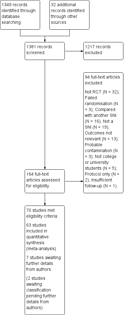
Study flow diagram.
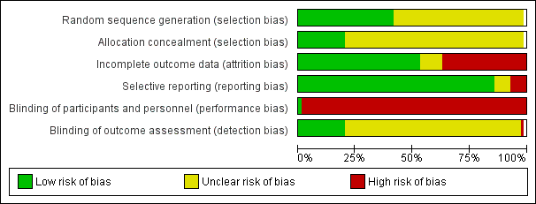
Methodological quality graph: review authors' judgements about each methodological quality item presented as percentages across all included studies.

Methodological quality summary: review authors' judgements about each methodological quality item for each included study.

Funnel plot of comparison: 1 Social norms (SN) vs control, outcome: 1.2 Alcohol‐related problems: 4+ months.

Funnel plot of comparison: 1 Social norms (SN) vs control, outcome: 1.4 Binge drinking: 4+ months.
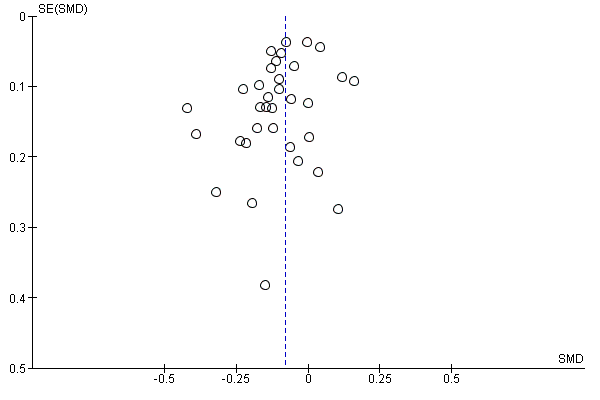
Funnel plot of comparison: 1 Social norms (SN) vs control, outcome: 1.6 Quantity of drinking: 4+ months.

Funnel plot of comparison: 1 Social norms (SN) vs control, outcome: 1.8 Frequency: 4+ months.
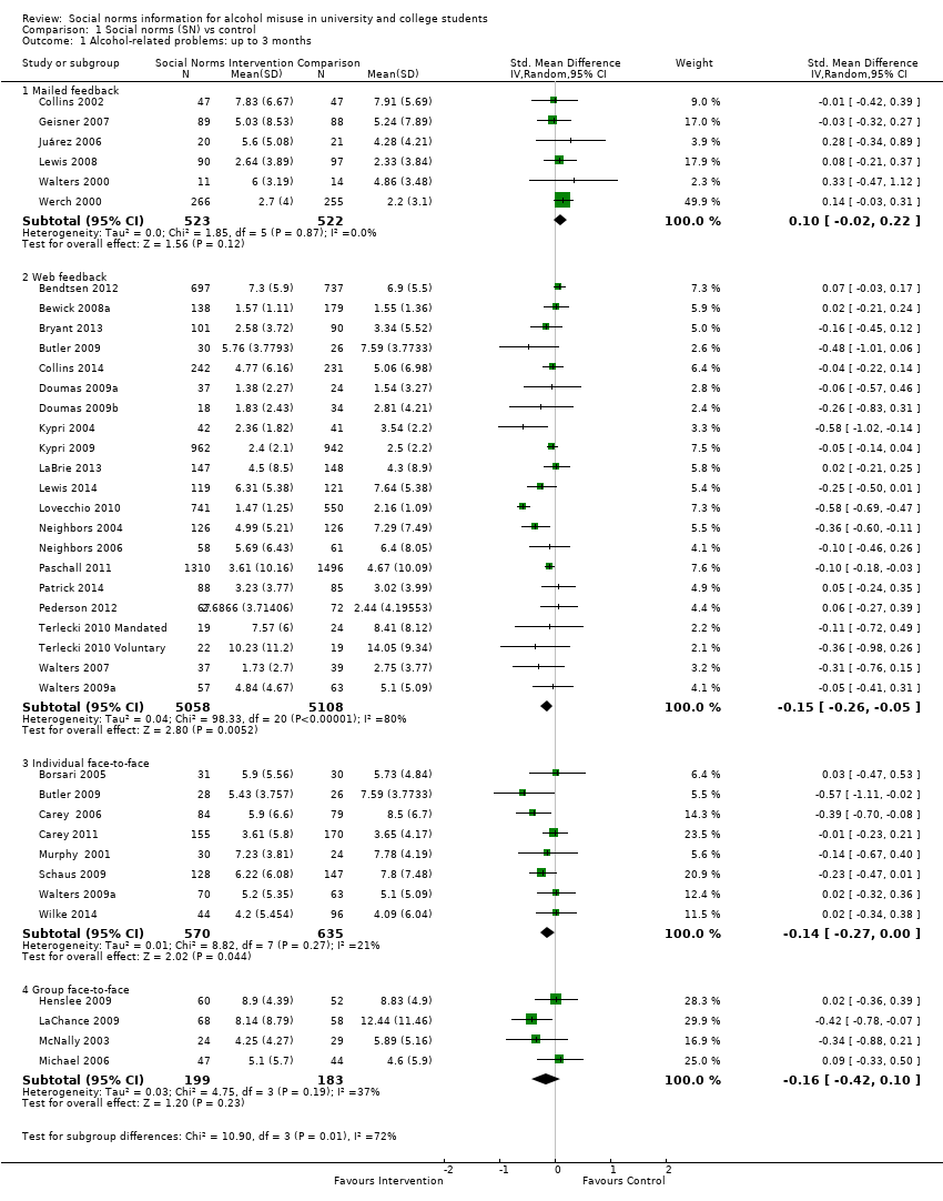
Comparison 1 Social norms (SN) vs control, Outcome 1 Alcohol‐related problems: up to 3 months.
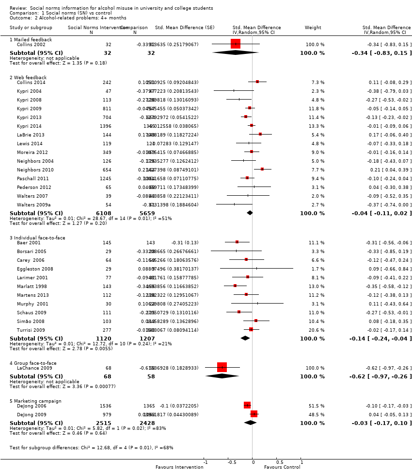
Comparison 1 Social norms (SN) vs control, Outcome 2 Alcohol‐related problems: 4+ months.
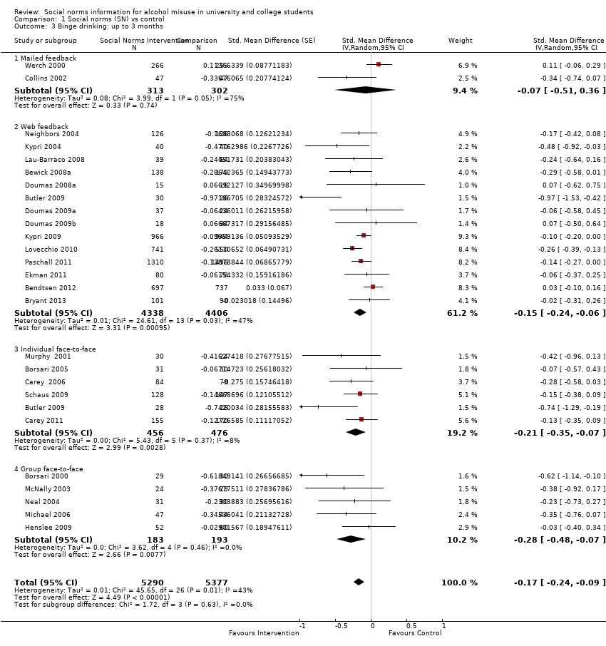
Comparison 1 Social norms (SN) vs control, Outcome 3 Binge drinking: up to 3 months.

Comparison 1 Social norms (SN) vs control, Outcome 4 Binge drinking: 4+ months.

Comparison 1 Social norms (SN) vs control, Outcome 5 Quantity of drinking: up to 3 months.

Comparison 1 Social norms (SN) vs control, Outcome 6 Quantity of drinking: 4+ months.

Comparison 1 Social norms (SN) vs control, Outcome 7 Frequency: up to 3 months.

Comparison 1 Social norms (SN) vs control, Outcome 8 Frequency: 4+ months.

Comparison 1 Social norms (SN) vs control, Outcome 9 Peak BAC: up to 3 months.

Comparison 1 Social norms (SN) vs control, Outcome 10 Peak BAC: 4+ months.

Comparison 1 Social norms (SN) vs control, Outcome 11 Typical BAC: up to 3 months.

Comparison 1 Social norms (SN) vs control, Outcome 12 Typical BAC: 4+ months.
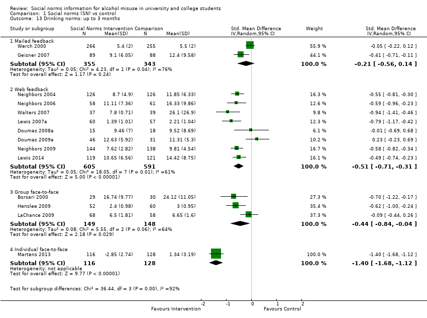
Comparison 1 Social norms (SN) vs control, Outcome 13 Drinking norms: up to 3 months.

Comparison 1 Social norms (SN) vs control, Outcome 14 Drinking norms: 4+ months.
| Social norms information compared with controls for prevention of alcohol misuse | ||||||
| Patient or population: university or college students Settings: college or university settings Intervention: social norms information (personalised feedback or information campaigns); by delivery mode if subgroup differences were noted between different delivery modes (mailed normative feedback; web/computer feedback; individual face‐to‐face feedback; group face‐to‐face feedback) Comparison: no intervention (assessment only or alcohol information or alternative (non‐normative) intervention) Follow‐up: 4+ months Measurement: self‐reported alcohol consumption (questionnaire scale) | ||||||
| Outcomes | Illustrative comparative risks* (95% CI) | Relative effect | Number of participants | Quality of the evidence | Comments | |
| Assumed risk | Corresponding risk | |||||
| Alcohol‐related problems: 4+ months—web/computer normative feedback | Mean alcohol problems scale score was 8.91 in the control group, with a standard deviation of 9.17 (the 69‐point RAPI scale was used by Martens 2013) | The SMD from the meta‐analysis (‐0.04) will result in a decrease of 0.37 in the alcohol problems scale score (95% CI 0.18 to 1.00), from an average of 8.91 to 8.54, based on Martens 2013 | (SMD ‐0.04, 95% CI ‐0.11 to 0.02) | 11,767 (15) | ⊕⊕⊝⊝ | Limitations in design and implementation, especially blinding and in some studies high risk of attrition bias (loss to follow‐up). Borderline substantial heterogeneity (I2 = 51%) |
| Alcohol‐related problems: 4+ months—individual face‐to‐face normative feedback | Mean alcohol problems scale score was 8.91 in the control group, with a standard deviation of 9.17 (the 69‐point RAPI scale was used by Martens 2013) | The SMD from the meta‐analysis (‐0.15) will result in a decrease of 1.28 in the alcohol problems scale score (95% CI 0.37 to 2.20), from an average of 8.91 to 7.63, based on Martens 2013 | (SMD ‐0.14, 95% CI ‐0.24 to ‐0.04) | 2327 (11) | ⊕⊕⊕⊝ | Limitations in design and implementation, especially blinding and in some studies high risk of attrition bias (loss to follow‐up) |
| Binge drinking: 4+ months (all delivery modes) | 43.9% of control group participants were binge drinkers, defined as those who drink above recommended limits for acute risk (> 40 g/> 60 g ethanol on 1 occasion in the preceding 4 weeks for women and men, respectively) in a study by Kypri 2014 | The SMD from the meta‐analysis (‐0.06) will result in 2.7% fewer binge drinkers (95% CI 0.9% to 4.8%), from 43.9% to 41.2%, based on Kypri 2014 | (SMD ‐0.06, 95% CI ‐0.11 to ‐0.02) | 11,292 (16) | ⊕⊕⊕⊝ | Limitations in design and implementation, especially blinding and in some studies high risk of attrition bias (loss to follow‐up) |
| Quantity of drinking: 4+ months (all delivery modes) | Mean number of drinks per week was 13.74 in the control group, with a standard deviation of 10.77, from the DDQ measure in Martens 2013 | The SMD from the meta‐analysis (‐0.08) will result in a decrease of 0.9 drinks consumed each week (95% CI 0.4 to 1.3), from an average of 13.7 drinks per week to 12.8 drinks per week, based on Martens 2013 | (SMD ‐0.08, 95% CI ‐0.12 to ‐0.04) | 21,169 (32) | ⊕⊕⊕⊝ | Limitations in design and implementation, especially blinding and in some studies high risk of attrition bias (loss to follow‐up) |
| Frequency: 4+ months—web/computer normative feedback | Mean number of drinking days per week was 2.74 in the control group, with a standard deviation of 1.54, from the DDQ measure in Martens 2013 | The SMD from the meta‐analysis (‐0.11) will result in a decrease of 0.17 drinking days per week (95% CI 0.06 to 0.26), from an average of 2.74 drinking days per week to 2.57 drinking days per week, based on Martens 2013 | (SMD ‐0.11, 95% CI ‐0.17 to ‐0.04) | 9929 (10) | ⊕⊕⊕⊝ | Limitations in design and implementation, especially blinding and in some studies high risk of attrition bias (loss to follow‐up) |
| Frequency: 4+ months—individual face‐to‐face normative feedback | Mean number of drinking days per week was 2.74 in the control group, with a standard deviation of 1.54, from the DDQ measure in Martens 2013 | The SMD from the meta‐analysis (‐0.21) will result in a decrease of 0.32 drinking days per week (95% CI 0.15 to 0.48), from an average of 2.74 drinking days per week to 2.42 drinking days per week, based on Martens 2013 | (SMD ‐0.21, 95% CI ‐0.31 to ‐0.10) | 1464 (8) | ⊕⊕⊕⊝ | Limitations in design and implementation, especially blinding and in some studies high risk of attrition bias (loss to follow‐up) |
| Frequency: 4+ months—group face‐to‐face normative feedback | Mean number of drinking days per week was 2.74 in the control group, with a standard deviation of 1.54, from the DDQ measure in Martens 2013 | The SMD from the meta‐analysis (‐0.26) will result in a decrease of 0.40 drinking days per week (95% CI 0.03 to 0.83), from an average of 2.74 drinking days per week to 2.34 drinking days per week, based on Martens 2013 | (SMD ‐0.26, 95% CI ‐0.54 to 0.02) | 449 (5) | ⊕⊕⊝⊝ | Limitations in design and implementation, especially blinding and in some studies high risk of attrition bias (loss to follow‐up). Substantial heterogeneity (I2 = 55%) |
| Peak BAC: 4+ months (all delivery modes) | Mean peak BAC was 0.144% in the control group, with a standard deviation of 0.111, from Martens 2013 | The SMD from the meta‐analysis (‐0.08) will result in a decrease of 0.009 for peak BAC (95% CI 0.000 to 0.019), from an average of 0.144% to 0.135%, based on Martens 2013 | (SMD ‐0.08, 95% CI ‐0.17 to 0.00) | 7198 (11) | ⊕⊕⊝⊝ | Limitations in design and implementation, especially blinding and in some studies high risk of attrition bias (loss to follow‐up). Borderline substantial heterogeneity (I2 = 50%) |
| Typical BAC: 4+ months—individual face‐to‐face normative feedback | Mean typical BAC was 0.08% in the control group, with a standard deviation of 0.048, from Schaus 2009 | The SMD from the meta‐analysis (‐0.08) will result in a decrease of 0.004 for typical BAC (95% CI ‐0.005 to 0.013), from an average of 0.080% to 0.076%, based on Schaus 2009 | (SMD ‐0.08, 95% CI ‐0.26 to 0.10) | 490 (4) | ⊕⊕⊕⊝ | Limitations in design and implementation, especially blinding and in some studies high risk of attrition bias (loss to follow‐up) |
| *The basis for the assumed risk is provided in footnotes. The corresponding risk (and its 95% confidence interval) is based on the assumed risk in the comparison group and the relative effect of the intervention (and its 95% CI). | ||||||
| GRADE Working Group grades of evidence. | ||||||
| In the columns illustrating comparative risks: for outcomes where the pooled analysis point estimate and confidence interval showed some effect, we have used results (mean scores and standard deviations) from Martens 2013 to illustrate the effect sizes in terms of the measures used in that study. We chose Martens 2013 because the outcome measures they use are well‐known, generally well regarded, and are typical of the measures used in this field of research: they used the Daily Drinking Questionnaire (DDQ) and the Rutgers Alcohol Problem Index (RAPI). | ||||||
| Outcome or subgroup title | No. of studies | No. of participants | Statistical method | Effect size |
| 1 Alcohol‐related problems: up to 3 months Show forest plot | 37 | Std. Mean Difference (IV, Random, 95% CI) | Subtotals only | |
| 1.1 Mailed feedback | 6 | 1045 | Std. Mean Difference (IV, Random, 95% CI) | 0.10 [‐0.02, 0.22] |
| 1.2 Web feedback | 21 | 10166 | Std. Mean Difference (IV, Random, 95% CI) | ‐0.15 [‐0.26, ‐0.05] |
| 1.3 Individual face‐to‐face | 8 | 1205 | Std. Mean Difference (IV, Random, 95% CI) | ‐0.14 [‐0.27, ‐0.00] |
| 1.4 Group face‐to‐face | 4 | 382 | Std. Mean Difference (IV, Random, 95% CI) | ‐0.16 [‐0.42, 0.10] |
| 2 Alcohol‐related problems: 4+ months Show forest plot | 30 | Std. Mean Difference (Random, 95% CI) | Subtotals only | |
| 2.1 Mailed feedback | 1 | 64 | Std. Mean Difference (Random, 95% CI) | ‐0.34 [‐0.83, 0.15] |
| 2.2 Web feedback | 15 | 11767 | Std. Mean Difference (Random, 95% CI) | ‐0.04 [‐0.11, 0.02] |
| 2.3 Individual face‐to‐face | 11 | 2327 | Std. Mean Difference (Random, 95% CI) | ‐0.14 [‐0.24, ‐0.04] |
| 2.4 Group face‐to‐face | 1 | 126 | Std. Mean Difference (Random, 95% CI) | ‐0.62 [‐0.97, ‐0.26] |
| 2.5 Marketing campaign | 2 | 4943 | Std. Mean Difference (Random, 95% CI) | ‐0.03 [‐0.17, 0.10] |
| 3 Binge drinking: up to 3 months Show forest plot | 26 | 10667 | Std. Mean Difference (Random, 95% CI) | ‐0.17 [‐0.24, ‐0.09] |
| 3.1 Mailed feedback | 2 | 615 | Std. Mean Difference (Random, 95% CI) | ‐0.07 [‐0.51, 0.36] |
| 3.2 Web feedback | 14 | 8744 | Std. Mean Difference (Random, 95% CI) | ‐0.15 [‐0.24, ‐0.06] |
| 3.3 Individual face‐to‐face | 6 | 932 | Std. Mean Difference (Random, 95% CI) | ‐0.21 [‐0.35, ‐0.07] |
| 3.4 Group face‐to‐face | 5 | 376 | Std. Mean Difference (Random, 95% CI) | ‐0.28 [‐0.48, ‐0.07] |
| 4 Binge drinking: 4+ months Show forest plot | 16 | 11292 | Std. Mean Difference (Random, 95% CI) | ‐0.06 [‐0.11, ‐0.02] |
| 4.1 Mailed feedback | 1 | 65 | Std. Mean Difference (Random, 95% CI) | ‐0.17 [‐0.66, 0.32] |
| 4.2 Web feedback | 10 | 10719 | Std. Mean Difference (Random, 95% CI) | ‐0.07 [‐0.12, ‐0.02] |
| 4.3 Individual face‐to‐face | 5 | 508 | Std. Mean Difference (Random, 95% CI) | 0.01 [‐0.17, 0.18] |
| 5 Quantity of drinking: up to 3 months Show forest plot | 45 | 14184 | Std. Mean Difference (IV, Random, 95% CI) | ‐0.14 [‐0.19, ‐0.09] |
| 5.1 Mailed feedback | 5 | 1020 | Std. Mean Difference (IV, Random, 95% CI) | ‐0.04 [‐0.21, 0.13] |
| 5.2 Web feedback | 28 | 10889 | Std. Mean Difference (IV, Random, 95% CI) | ‐0.12 [‐0.18, ‐0.07] |
| 5.3 Individual face‐to‐face | 8 | 1309 | Std. Mean Difference (IV, Random, 95% CI) | ‐0.24 [‐0.38, ‐0.11] |
| 5.4 Group face‐to‐face | 5 | 411 | Std. Mean Difference (IV, Random, 95% CI) | ‐0.30 [‐0.49, ‐0.10] |
| 5.5 Marketing campaign | 1 | 555 | Std. Mean Difference (IV, Random, 95% CI) | ‐0.05 [‐0.22, 0.11] |
| 6 Quantity of drinking: 4+ months Show forest plot | 32 | 21169 | Std. Mean Difference (Random, 95% CI) | ‐0.08 [‐0.12, ‐0.04] |
| 6.1 Mailed feedback | 2 | 533 | Std. Mean Difference (Random, 95% CI) | ‐0.13 [‐0.32, 0.06] |
| 6.2 Web feedback | 18 | 13319 | Std. Mean Difference (Random, 95% CI) | ‐0.07 [‐0.12, ‐0.02] |
| 6.3 Individual face‐to‐face | 12 | 2374 | Std. Mean Difference (Random, 95% CI) | ‐0.15 [‐0.23, ‐0.08] |
| 6.4 Marketing campaign | 2 | 4943 | Std. Mean Difference (Random, 95% CI) | ‐0.02 [‐0.13, 0.09] |
| 7 Frequency: up to 3 months Show forest plot | 19 | Std. Mean Difference (IV, Random, 95% CI) | Subtotals only | |
| 7.1 Mailed feedback | 1 | 521 | Std. Mean Difference (IV, Random, 95% CI) | 0.12 [‐0.05, 0.29] |
| 7.2 Web feedback | 12 | 6385 | Std. Mean Difference (IV, Random, 95% CI) | ‐0.17 [‐0.25, ‐0.09] |
| 7.3 Individual face‐to‐face | 4 | 515 | Std. Mean Difference (IV, Random, 95% CI) | ‐0.45 [‐0.63, ‐0.28] |
| 7.4 Group face‐to‐face | 3 | 264 | Std. Mean Difference (IV, Random, 95% CI) | ‐0.03 [‐0.27, 0.21] |
| 8 Frequency: 4+ months Show forest plot | 25 | Std. Mean Difference (Random, 95% CI) | Subtotals only | |
| 8.1 Web feedback | 10 | 9929 | Std. Mean Difference (Random, 95% CI) | ‐0.11 [‐0.17, ‐0.04] |
| 8.2 Individual face‐to‐face | 8 | 1464 | Std. Mean Difference (Random, 95% CI) | ‐0.21 [‐0.31, ‐0.10] |
| 8.3 Group face‐to‐face | 5 | 449 | Std. Mean Difference (Random, 95% CI) | ‐0.26 [‐0.54, 0.02] |
| 8.4 Marketing campaign | 2 | 4943 | Std. Mean Difference (Random, 95% CI) | ‐0.01 [‐0.09, 0.06] |
| 9 Peak BAC: up to 3 months Show forest plot | 11 | 1902 | Std. Mean Difference (IV, Random, 95% CI) | ‐0.22 [‐0.33, ‐0.11] |
| 9.1 Mailed feedback | 1 | 94 | Std. Mean Difference (IV, Random, 95% CI) | ‐0.20 [‐0.60, 0.21] |
| 9.2 Web feedback | 4 | 477 | Std. Mean Difference (IV, Random, 95% CI) | ‐0.13 [‐0.35, 0.09] |
| 9.3 Individual face‐to‐face | 7 | 1331 | Std. Mean Difference (IV, Random, 95% CI) | ‐0.26 [‐0.39, ‐0.13] |
| 10 Peak BAC: 4+ months Show forest plot | 11 | 7198 | Std. Mean Difference (IV, Random, 95% CI) | ‐0.08 [‐0.17, 0.00] |
| 10.1 Mailed feedback | 1 | 468 | Std. Mean Difference (IV, Random, 95% CI) | ‐0.13 [‐0.33, 0.08] |
| 10.2 Web feedback | 3 | 355 | Std. Mean Difference (IV, Random, 95% CI) | ‐0.08 [‐0.29, 0.13] |
| 10.3 Individual face‐to‐face | 7 | 1432 | Std. Mean Difference (IV, Random, 95% CI) | ‐0.16 [‐0.26, ‐0.05] |
| 10.4 Marketing campaign | 2 | 4943 | Std. Mean Difference (IV, Random, 95% CI) | 0.02 [‐0.18, 0.21] |
| 11 Typical BAC: up to 3 months Show forest plot | 8 | 1336 | Std. Mean Difference (IV, Random, 95% CI) | ‐0.17 [‐0.31, ‐0.03] |
| 11.1 Mailed feedback | 3 | 253 | Std. Mean Difference (IV, Random, 95% CI) | ‐0.10 [‐0.35, 0.15] |
| 11.2 Web feedback | 1 | 282 | Std. Mean Difference (IV, Random, 95% CI) | ‐0.25 [‐0.48, ‐0.01] |
| 11.3 Individual face‐to‐face | 4 | 801 | Std. Mean Difference (IV, Random, 95% CI) | ‐0.14 [‐0.40, 0.12] |
| 12 Typical BAC: 4+ months Show forest plot | 4 | Std. Mean Difference (IV, Random, 95% CI) | Subtotals only | |
| 12.1 Individual face‐to‐face | 4 | 490 | Std. Mean Difference (IV, Random, 95% CI) | ‐0.08 [‐0.26, 0.10] |
| 13 Drinking norms: up to 3 months Show forest plot | 14 | Std. Mean Difference (IV, Random, 95% CI) | Subtotals only | |
| 13.1 Mailed feedback | 2 | 698 | Std. Mean Difference (IV, Random, 95% CI) | ‐0.21 [‐0.56, 0.14] |
| 13.2 Web feedback | 8 | 1196 | Std. Mean Difference (IV, Random, 95% CI) | ‐0.51 [‐0.71, ‐0.31] |
| 13.3 Group face‐to‐face | 3 | 297 | Std. Mean Difference (IV, Random, 95% CI) | ‐0.44 [‐0.84, ‐0.04] |
| 13.4 Individual face‐to‐face | 1 | 244 | Std. Mean Difference (IV, Random, 95% CI) | ‐1.40 [‐1.68, ‐1.12] |
| 14 Drinking norms: 4+ months Show forest plot | 9 | Std. Mean Difference (Random, 95% CI) | Subtotals only | |
| 14.1 Web feedback | 6 | 2227 | Std. Mean Difference (Random, 95% CI) | ‐0.34 [‐0.57, ‐0.11] |
| 14.2 Individual face‐to‐face | 1 | 240 | Std. Mean Difference (Random, 95% CI) | ‐1.19 [‐1.47, ‐0.92] |
| 14.3 Marketing campaign | 2 | 4943 | Std. Mean Difference (Random, 95% CI) | ‐0.06 [‐0.23, 0.11] |